Hello!

Welcome back. Today, we will be building off of the concepts and research in the last post.

We will cover the sources of return for our strategy, potential filters to use in the strategy, and a high-performing initial iteration of the strategy.

We will likely have a third post on this topic, due to the interest from paid subscribers. The code has been sent to your emails.

Let’s get into it.

Volatility Decay Recap

Our first post establishes the mathematical foundation for understanding volatility decay and optimal leverage in the U.S. equity markets. It begins by distinguishing between Arithmetic Mean (simple average) and Geometric Growth (compounded wealth), noting that while statistical models often prefer the former, investors care about the latter.

We utilize a Taylor Series approximation to mathematically model geometric returns (ln(1+x)), deriving the specific formula for volatility drag (decay): -(σ^2)/2. This proves that volatility is a direct penalty to compounded returns. We then extend this math to a leveraged portfolio, deriving a formula that balances excess returns against the accelerating drag of leverage. Finally, by optimizing this formula (finding the derivative and setting it to zero), we arrive at the Kelly Criterion, calculating that the historical “Optimal Leverage” for the S&P 500 is approximately 2.13x.

I also shared a research paper that covered a simple, high-Sharpe strategy to harvest this decay.

Implications of Kurtosis and Skew

In the previous post, I made a convenient assumption in the beginning. I assumed stock returns are normally distributed (a bell curve). This is a standard assumption in finance (as it is in the Black-Scholes model), but we know it is incorrect. If the market were truly “Normal,” a 3-standard deviation crash (a massive outlier) would happen roughly once every 7,000 years. In reality, we see them every decade.

To find the true cost of leverage, we have to look beyond the Mean and Variance (the first two terms in the Taylor series expansion). We need to expand our Taylor Series approximation to include the 3rd and 4th moments of the distribution: Skewness and Kurtosis. In the last post, I simply stopped after the first two terms, due to the difficulty to incorporate all the information and to focus in on the core concepts of volatility decay and LETF behavior.

When we expand the series, the formula for Geometric Growth changes from a simple variance penalty (-(σ^2)/2) to this:

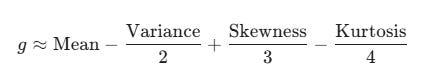
Skewness measures the asymmetry of returns. While a normal distribution has zero skew, the stock market exhibits negative skew, meaning it tends to crash faster than it rallies. In our expanded formula, the skew term is technically added (positive), but because market skewness is negative, this term effectively becomes a subtraction (negative), creating a drag on compound returns.

Similarly, Kurtosis measures the “fatness” of the tails, or how often extreme events occur. The market is leptokurtic, meaning it has fat tails. Since the formula subtracts kurtosis and market kurtosis is high, this creates another significant penalty to growth.

The math becomes particularly punishing when leverage is applied because these penalties do not scale linearly. Instead, they scale according to the power of the moment.

While the mean return scales linearly with leverage (f), variance scales quadratically (f2), skewness scales cubically (f3), and kurtosis scales quartically (f4). This means that for a 3x leveraged ETF, the investor is not simply taking on three times the risk. They are exposing the portfolio to nine times the variance drag, twenty-seven times the skewness risk, and eighty-one times the kurtosis risk.

This accelerated decay explains why theoretical optimal leverage models, which often ignore these higher moments, tend to overestimate the amount of leverage a portfolio can actually withstand during a crisis.

Autocorrelation

Another assumption hidden in standard volatility models is that returns are “independent.” This means that what happened yesterday has zero influence on what happens today (like flipping a coin).

If the market were truly a series of independent coin flips, volatility would scale perfectly with time, and our standard decay formula would be precise. However, we know that markets often have memory. In reality, returns are often correlated with their past selves. This is called autocorrelation.

When the market exhibits positive autocorrelation, it is trending. A big up day is (more) likely to be followed by another up day (rather than a negative day). This persistence smooths out the path of the asset, suppressing the actual realized volatility relative to the daily noise.

This explains why leveraged ETFs can perform exceptionally well in steady, low-volatility bull markets (like 2017); the trend effectively fights back against the decay, allowing the compounding to work more efficiently.

Conversely, negative autocorrelation creates a nightmare scenario for leverage. This occurs when the market “chops” or mean-reverts. In this case, a big up day is (more) likely to be followed by a big down day, and vice versa. This constant whipsawing forces a leveraged fund to repeatedly buy high and sell low (short gamma, anyone?) just to maintain its target leverage ratio.

In this environment, volatility decay is amplified significantly beyond what the variance formula predicts, destroying value much faster. This helps explain why choppy bear markets (like 2022) are destructive to LETFs.

LETF Swap Costs

Lastly, we need to cover the inherent costs to set up and manage these LETFs. While most investors focus on the expense ratio, the primary cost is structural. To achieve 3x exposure, these funds utilize Total Return Swaps. While the fund does not literally borrow cash to purchase shares, the swap agreement requires them to pay a financing rate to the counterparty (typically SOFR + spread) in exchange for the leveraged exposure.

In a zero-interest-rate environment, this cost is negligible, but in a world with 4% rates, it becomes a significant daily drag on the fund’s Net Asset Value.

This financing cost creates a “hurdle rate” for the fund. The underlying index cannot simply stay flat; it must rise enough to cover the financing bill before the ETF generates a positive return.

Bull funds are forced to pay this high financing rate, which accelerates their value erosion. Bear funds, conversely, often receive interest on their short exposure, which offsets some of their volatility decay.

When you short a Bull ETF, you are capturing both the volatility decay and the financing costs the fund is forced to pay.

With interest rates currently high, this is another (and significant) tailwind for our strategy, as you will see below. Let’s dive into the backtested strategy.