この記事はどんな記事なのだ?
こんにちはなのだ、kaggle masterのアライさんなのだ。
この記事はkaggle advent calendar 2019 その1の13日目の記事なのだ。
前日はu++さんのKaggle Days Tokyoの記事なのだ。アライさんも参加したかったのだ。
明日はtakapy0210さんの学習・推論パイプラインについてなのだ。楽しみなのだ。
Kagglerの間では連綿と受け継がれる便利関数がいくつかあるのだ。アライさんはそれをKaggleコード遺産と呼ぶことにしたのだ。この記事ではKaggleコード遺産の紹介とその出処の検証1を行おうと思うのだ。面白かったら是非upvoteしてくださいなのだ。
さあKaggleパークの冒険に出発なのだ!
おことわり
今回の記事はPythonコードに限った話になってしまったのだ。KaggleのNotebookではRも使えるようになっているけれど、アライさんはRは使えないのだ。Rコードでもコード遺産があるなら教えて欲しいのだ。
Kaggleコード遺産
utility遺産
ここではKaggleで一般的に使われるutility関数たちを紹介するのだ!
timer
みんな大好き、timerなのだ。時間を図るのが得意な関数2なのだ。
import time

from contextlib import contextmanager


@contextmanager
def timer(name):
    t0 = time.time()
    yield
    print(f'[{name}] done in {time.time() - t0:.0f} s')
with文で使うとwithブロック内の計算の実行時間を測ってくれるのだ。
def wait(sec: float):
    time.sleep(sec)


with timer("wait"):
    wait(2.0)


# => [wait] done in 2 s
初出はたぶん、Mercari Price Suggestion Challengeの一位、Lopuhinさんの解法なのだ。Lopuhinさんの解法は非常に簡潔で過去のコンペの解法の中でも特に有名なやつなのだ。
このコンペは初めてのカーネルonlyコンペで計算時間制限もCPUで1hourと非常に厳しい条件が課せられていたのだ。そのせいもあってコンペの期間中からスクリプト中の各パートの計算時間を計測してボトルネックを把握するのが流行っていたのだ。例えば、高スコアを出していたこのカーネル中では、
start_time = time.time()
# (中略)
handle_missing_inplace(merge)
print('[{}] Finished to handle missing'.format(time.time() - start_time))
みたいなコードが散見されるのだ。Lopuhinさんのtimerはこれをcontextmanagerを使って
もう少しエレガントにしたものなのだ。
ちなみにメルカリコンペはアライさんが初めて参加したコンペなので思い出深いコンペなのだ。良コンペなのでみんなlateサブをしてみるのだ。
こういったコード遺産はみんなに使われていくうちにちょっとずつバリエーションが出てくるものなのだ。次の例は、Petfinder Adoption Predictionの2位解法で使われている例なのだ。
@contextmanager
def timer(name):
    t0 = time.time()
    yield
    logger.info(f'[{name}] done in {time.time() - t0:.0f} s')
この例では、loggerオブジェクトをglobalで定義しておいてlogに吐くようにしているのだ。アライさんは
import logging

from typing import Optional


@contextmanager
def timer(name: str, logger: Optional[logging.Logger] = None):
    t0 = time.time()
    yield
    msg = f"[{name}] done in {time.time()-t0:.0f} s"
    if logger:
        logger.info(msg)
    else:
        print(msg)
を使っているのだ。loggerを渡した時と渡さないときで挙動を変えるようにしているのだ。
ちなみにあまり流行らなかったけれど、Mercariコンペより前に似たような発想のtimerが世に出ていたようなのだ。このカーネル中では
import cv2
import datetime
import time


def time_function_execution(function_to_execute):
    def compute_execution_time(*args, **kwargs):
        start_time = time.time()
        result = function_to_execute(*args, **kwargs)
        end_time = time.time()
        computation_time = datetime.timedelta(seconds=end_time - start_time)
        print('I am done!')
        print('Computation lasted: {}'.format(computation_time))
        return result
    return compute_execution_time


## Time the loading of all training files (normal and in parallel)

def load_image(img_file):
    return cv2.imread(img_file)

@time_function_execution
def load_images(img_files):
    imgs = []
    for img_file in img_files:
        imgs.append(load_image(img_file))
    return imgs
time_function_executionというデコレータが使われているのだ。なかなか興味深いのだ。
reduce_mem_usage
メモリ使用量を減らすのが得意な関数なのだ。でもアライさんは使ったことがないのだ。
今現在よく使われているのはHome Credit Default Riskの時にこのカーネルで紹介されていたバージョンのようなのだ。
import numpy as np
import pandas as pd


def reduce_mem_usage(df):
    """ iterate through all the columns of a dataframe and modify the data type
        to reduce memory usage.
    """
    start_mem = df.memory_usage().sum() / 1024**2
    print('Memory usage of dataframe is {:.2f} MB'.format(start_mem))

    for col in df.columns:
        col_type = df[col].dtype

        if col_type != object:
            c_min = df[col].min()
            c_max = df[col].max()
            if str(col_type)[:3] == 'int':
                if c_min > np.iinfo(np.int8).min and c_max < np.iinfo(np.int8).max:
                    df[col] = df[col].astype(np.int8)
                elif c_min > np.iinfo(np.int16).min and c_max < np.iinfo(np.int16).max:
                    df[col] = df[col].astype(np.int16)
                elif c_min > np.iinfo(np.int32).min and c_max < np.iinfo(np.int32).max:
                    df[col] = df[col].astype(np.int32)
                elif c_min > np.iinfo(np.int64).min and c_max < np.iinfo(np.int64).max:
                    df[col] = df[col].astype(np.int64)
            else:
                if c_min > np.finfo(np.float16).min and c_max < np.finfo(np.float16).max:
                    df[col] = df[col].astype(np.float16)
                elif c_min > np.finfo(np.float32).min and c_max < np.finfo(np.float32).max:
                    df[col] = df[col].astype(np.float32)
                else:
                    df[col] = df[col].astype(np.float64)
        else:
            df[col] = df[col].astype('category')

    end_mem = df.memory_usage().sum() / 1024**2
    print('Memory usage after optimization is: {:.2f} MB'.format(end_mem))
    print('Decreased by {:.1f}%'.format(100 * (start_mem - end_mem) / start_mem))

    return df
ちょっと長いけどやっていることは単純で、より低い精度の型で表現できるなら精度を落とした型を使おうという発想なのだ。
先述のカーネル中ではZillow Prize: Zillow's Home Value Predictionで紹介されたこのカーネルを参考にしたという記述があるのだ。なのでたぶん、reduce_mem_usageの初出はこれなのだ。
def reduce_mem_usage(props):
    start_mem_usg = props.memory_usage().sum() / 1024**2
    print("Memory usage of properties dataframe is :",start_mem_usg," MB")
    NAlist = [] # Keeps track of columns that have missing values filled in.
    for col in props.columns:
        if props[col].dtype != object:  # Exclude strings

            # Print current column type
            print("******************************")
            print("Column: ",col)
            print("dtype before: ",props[col].dtype)

            # make variables for Int, max and min
            IsInt = False
            mx = props[col].max()
            mn = props[col].min()

            # Integer does not support NA, therefore, NA needs to be filled
            if not np.isfinite(props[col]).all():
                NAlist.append(col)
                props[col].fillna(mn-1,inplace=True)

            # test if column can be converted to an integer
            asint = props[col].fillna(0).astype(np.int64)
            result = (props[col] - asint)
            result = result.sum()
            if result > -0.01 and result < 0.01:
                IsInt = True


            # Make Integer/unsigned Integer datatypes
            if IsInt:
                if mn >= 0:
                    if mx < 255:
                        props[col] = props[col].astype(np.uint8)
                    elif mx < 65535:
                        props[col] = props[col].astype(np.uint16)
                    elif mx < 4294967295:
                        props[col] = props[col].astype(np.uint32)
                    else:
                        props[col] = props[col].astype(np.uint64)
                else:
                    if mn > np.iinfo(np.int8).min and mx < np.iinfo(np.int8).max:
                        props[col] = props[col].astype(np.int8)
                    elif mn > np.iinfo(np.int16).min and mx < np.iinfo(np.int16).max:
                        props[col] = props[col].astype(np.int16)
                    elif mn > np.iinfo(np.int32).min and mx < np.iinfo(np.int32).max:
                        props[col] = props[col].astype(np.int32)
                    elif mn > np.iinfo(np.int64).min and mx < np.iinfo(np.int64).max:
                        props[col] = props[col].astype(np.int64)

            # Make float datatypes 32 bit
            else:
                props[col] = props[col].astype(np.float32)

            # Print new column type
            print("dtype after: ",props[col].dtype)
            print("******************************")

    # Print final result
    print("___MEMORY USAGE AFTER COMPLETION:___")
    mem_usg = props.memory_usage().sum() / 1024**2
    print("Memory usage is: ",mem_usg," MB")
    print("This is ",100*mem_usg/start_mem_usg,"% of the initial size")
    return props, NAlist
この中では欠損値処理とかもされているっぽいのだ。
seed_everything
乱数のseedを固定するやつなのだ。再現性の確保が得意な関数なのだ。
アライさんの記憶ではこの関数の初出はQuora Insincere Questions Classificationだったのだ。ただしこの時はseed_torchという名前だったのだ。
import os
import random

import numpy as np
import torch


def seed_torch(seed=1029):
    random.seed(seed)
    os.environ['PYTHONHASHSEED'] = str(seed)
    np.random.seed(seed)
    torch.manual_seed(seed)
    torch.cuda.manual_seed(seed)
    torch.backends.cudnn.deterministic = True
PyTorch, Tensorflow, Kerasなどのフレームワークを使わないのであれば、
def seed_everything(seed: int):
    random.seed(seed)
    os.environ["PYTHONHASHSEED"] = str(seed)
    np.random.seed(seed)
なのだ。逆にPyTorch, Tensorflowなどを使うことを想定しているのなら
import os
import random

import numpy as np
import tensorflow as tf
import torch


def seed_everything(seed=1234):
    random.seed(seed)
    os.environ['PYTHONHASHSEED'] = str(seed)
    np.random.seed(seed)
    tf.random.set_seed(seed)
    torch.manual_seed(seed)
    torch.cuda.manual_seed(seed)
    torch.backends.cudnn.deterministic = True
なのだ。ちなみにTensorflow2.0対応のコードなのだ。
visualization遺産
plot_confusion_matrix
Classificationのコンペではよく見かける、confusion matrixをきれいにしてくれるやつなのだ。初出はPLAsTiCC Astronomical Classificationなのだ。でもどれが最初に出したカーネルだったか見つけられなかったのだ。たしか運営が出したコードにあった気がするけどちょっと記憶が曖昧なのだ。
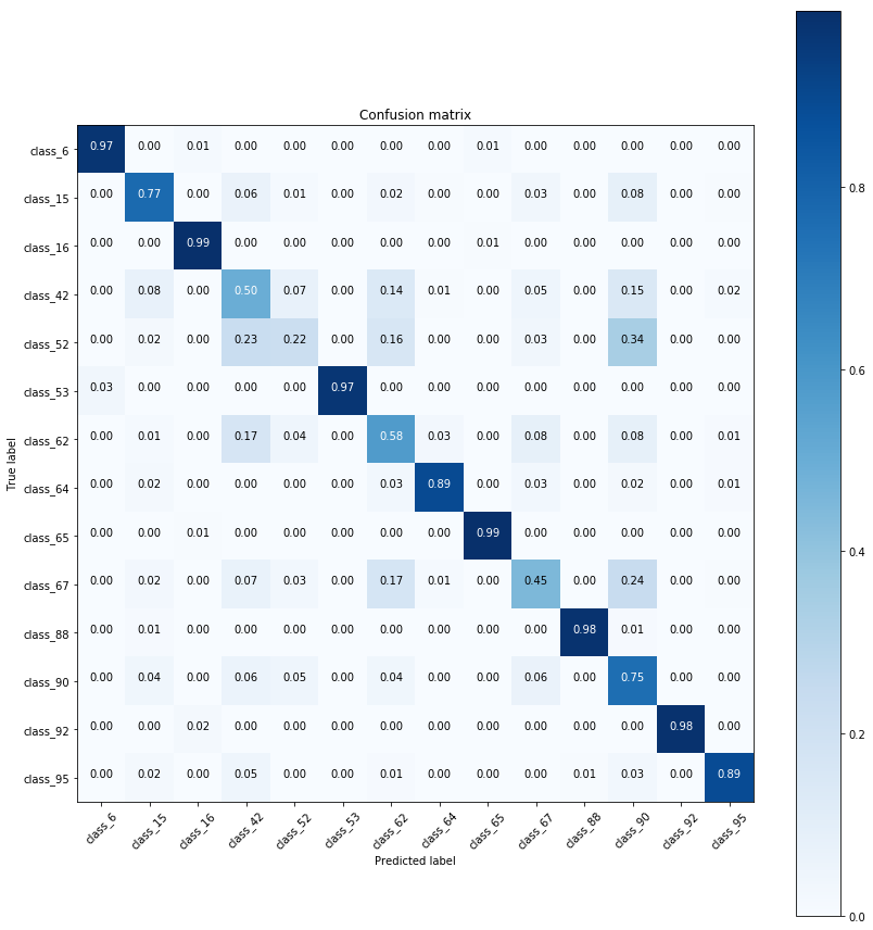
こんな感じの図が描けるやつなのだ。
import itertools

import matplotlib.pyplot as plt
import numpy as np


def plot_confusion_matrix(cm, classes,
                          normalize=False,
                          title='Confusion matrix',
                          cmap=plt.cm.Blues):
    if normalize:
        cm = cm.astype('float') / cm.sum(axis=1)[:, np.newaxis]
        print("Normalized confusion matrix")
    else:
        print('Confusion matrix, without normalization')

    print(cm)

    plt.imshow(cm, interpolation='nearest', cmap=cmap)
    plt.title(title)
    plt.colorbar()
    tick_marks = np.arange(len(classes))
    plt.xticks(tick_marks, classes, rotation=45)
    plt.yticks(tick_marks, classes)

    fmt = '.2f' if normalize else 'd'
    thresh = cm.max() / 2.
    for i, j in itertools.product(range(cm.shape[0]), range(cm.shape[1])):
        plt.text(j, i, format(cm[i, j], fmt),
                 horizontalalignment="center",
                 color="white" if cm[i, j] > thresh else "black")

    plt.ylabel('True label')
    plt.xlabel('Predicted label')
    plt.tight_layout()
使い方は、
from sklearn.metrics import confusion_matrix


cm = confusion_matrix(y_test, y_pred)
np.set_printoptions(precision=2)

class_names = np.unique(y_pred).tolist()


plt.figure(figsize=(5,5))
plot_confusion_matrix(
    cm,
    classes=class_names,
    normalize=True,
    title='Confusion matrix')
なのだ。最近これを使っていたらonoderaさんから
と言われてしまったのだ。onoderaさんverは表示がきれいなのでみんな使うのだ。
from mpl_toolkits.axes_grid1 import make_axes_locatable
from sklearn.utils.multiclass import unique_labels


def plot_confusion_matrix(y_true, y_pred, classes,
                          normalize=False,
                          title=None,
                          cmap=plt.cm.Blues):
    """
    Refer to: https://scikit-learn.org/stable/auto_examples/model_selection/plot_confusion_matrix.html

    This function prints and plots the confusion matrix.
    Normalization can be applied by setting `normalize=True`.
    """
    if not title:
        if normalize:
            title = 'Normalized confusion matrix'
        else:
            title = 'Confusion matrix, without normalization'

    # Compute confusion matrix
    cm = confusion_matrix(y_true, y_pred)
    # Only use the labels that appear in the data
    classes = classes[unique_labels(y_true, y_pred)]
    if normalize:
        cm = cm.astype('float') / cm.sum(axis=1)[:, np.newaxis]
        print("Normalized confusion matrix")
    else:
        print('Confusion matrix, without normalization')

    print(cm)

    fig, ax = plt.subplots(figsize=(10, 10))
    im = ax.imshow(cm, interpolation='nearest', cmap=cmap)
    tick_marks = np.arange(len(classes))
    plt.xticks(tick_marks, fontsize=25)
    plt.yticks(tick_marks, fontsize=25)
    plt.xlabel('Predicted label',fontsize=25)
    plt.ylabel('True label', fontsize=25)
    plt.title(title, fontsize=30)

    divider = make_axes_locatable(ax)
    cax = divider.append_axes('right', size="5%", pad=0.15)
    cbar = ax.figure.colorbar(im, ax=ax, cax=cax)
    cbar.ax.tick_params(labelsize=20)

    # We want to show all ticks...
    ax.set(xticks=np.arange(cm.shape[1]),
           yticks=np.arange(cm.shape[0]),
           # ... and label them with the respective list entries
           xticklabels=classes, yticklabels=classes,
#            title=title,
           ylabel='True label',
           xlabel='Predicted label')

    # Rotate the tick labels and set their alignment.
    plt.setp(ax.get_xticklabels(), ha="right",
             rotation_mode="anchor")

    # Loop over data dimensions and create text annotations.
    fmt = '.2f' if normalize else 'd'
    thresh = cm.max() / 2.
    for i in range(cm.shape[0]):
        for j in range(cm.shape[1]):
            ax.text(j, i, format(cm[i, j], fmt),
                    fontsize=20,
                    ha="center", va="center",
                    color="white" if cm[i, j] > thresh else "black")
    fig.tight_layout()
    return ax
ちなみにseabornでもほぼ同じ図が描けるのだ。
import seaborn as sns


fig, ax = plt.subplots(figsize=(9,7))
sns.heatmap(cm, xticklabels=labels, yticklabels=labels, cmap='Blues', annot=annot, lw=0.5)
ax.set_xlabel('Predicted Label')
ax.set_ylabel('True Label')
ax.set_aspect('equal')
plot_feature_importance
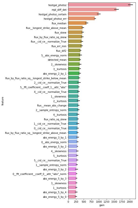
LightGBM, CatBoostなどのfeature importanceを綺麗に描画するやつなのだ。かなり昔から存在している気がするけどアライさんにはoriginalを見つけられなかったのだ。
そもそも関数として整えられていないことの方が多い気がするのだ。結果がこんな感じでカラフルになるやつを載せておくのだ。
import matplotlib.pyplot as plt
import pandas as pd
import seaborn as sns


def save_importances(importances_: pd.DataFrame):
    mean_gain = importances_[['gain', 'feature']].groupby('feature').mean()
    importances_['mean_gain'] = importances_['feature'].map(mean_gain['gain'])
    plt.figure(figsize=(8, 12))
    sns.barplot(
        x='gain',
        y='feature',
        data=importances_.sort_values('mean_gain', ascending=False)[:300])
    plt.tight_layout()
    plt.savefig('importances.png')
使い方としては
# fullはpandas.DataFrameなのだ。学習に使った特徴のDataFrameなのだ
# kfはsklearn.model_selection.KFoldのインスタンスなのだ
# clfはlightgbm.LGBMClassifierかlightgbm.LGBMRegressorだと思って欲しいのだ

importances = pd.DataFrame()

for fold_, (trn_idx, val_idx) in enumerate(kf.split(full)):
    # (中略)

    imp_df = pd.DataFrame()
    imp_df['feature'] = full.columns
    imp_df['gain'] = clf.feature_importances_
    imp_df['fold'] = fold_ + 1
    importances = pd.concat([importances, imp_df], axis=0, sort=False)


save_importances(importances)
なのだ。
metric遺産
特定の指標向けの最適化なんかのコード遺産なのだ。
threshold_search
二値分類問題で閾値最適化が得意な関数なのだ。
確率値ではなくて、0/1のクラスの予測を提出する必要がある時に使えるのだ。評価指標としてF1 score, Matthews Correlation Coefficient(MCC), Fβ scoreなんかが採用されているとき用なのだ。
初出はたぶん、Quora Insincere Question Classificationなのだ。このコンペの評価指標はF1 scoreだったのだ。
from sklearn.metrics import f1_score
from tqdm import tqdm


def threshold_search(y_true, y_proba):
    best_threshold = 0
    best_score = 0
    for threshold in tqdm([i * 0.01 for i in range(100)], disable=True):
        score = f1_score(y_true=y_true, y_pred=y_proba > threshold)
        if score > best_score:
            best_threshold = threshold
            best_score = score
    search_result = {'threshold': best_threshold, 'f1': best_score}
    return search_result
より一般化すると次みたいになるのだ。
import numpy as np

from typing import Callable, Dict


def threshold_search(
    y_true: np.ndarray,
    y_proba: np.ndarray,
    func: Callable[[np.ndarray, np.ndarray], float],
    is_higher_better: bool=True
) -> Dict[str, float]:
    best_threshold = 0.0
    best_score = -np.inf if is_higher_better else np.inf

    for threshold in [i * 0.01 for i in range(100)]:
        score = func(y_true=y_true, y_pred=y_pred > threshold)
        if is_higher_better:
            if score > best_score:
                best_threshold = threshold
                best_score = score
        else:
            if score < best_score:
                best_threshold = threshold
                best_score = score

    search_result = {
        "threshold": best_threshold,
        "score": best_score
    }
    return search_result
QWK
2019年に頻出したQuadratic Weighted Kappaの計算が得意な関数なのだ。
様々なバリエーションが存在するのだ。まずは2019年のQWKコンペのトップバッター、Petfinder.my Adoption Predictionの公開カーネルで紹介されていたものなのだ。
import numpy as np


# The following 3 functions have been taken from Ben Hamner's github repository
# https://github.com/benhamner/Metrics
def confusion_matrix(rater_a, rater_b, min_rating=None, max_rating=None):
    """
    Returns the confusion matrix between rater's ratings
    """
    assert(len(rater_a) == len(rater_b))
    if min_rating is None:
        min_rating = min(rater_a + rater_b)
    if max_rating is None:
        max_rating = max(rater_a + rater_b)
    num_ratings = int(max_rating - min_rating + 1)
    conf_mat = [[0 for i in range(num_ratings)]
                for j in range(num_ratings)]
    for a, b in zip(rater_a, rater_b):
        conf_mat[a - min_rating][b - min_rating] += 1
    return conf_mat


def histogram(ratings, min_rating=None, max_rating=None):
    """
    Returns the counts of each type of rating that a rater made
    """
    if min_rating is None:
        min_rating = min(ratings)
    if max_rating is None:
        max_rating = max(ratings)
    num_ratings = int(max_rating - min_rating + 1)
    hist_ratings = [0 for x in range(num_ratings)]
    for r in ratings:
        hist_ratings[r - min_rating] += 1
    return hist_ratings


def quadratic_weighted_kappa(y, y_pred):
    """
    Calculates the quadratic weighted kappa
    axquadratic_weighted_kappa calculates the quadratic weighted kappa
    value, which is a measure of inter-rater agreement between two raters
    that provide discrete numeric ratings.  Potential values range from -1
    (representing complete disagreement) to 1 (representing complete
    agreement).  A kappa value of 0 is expected if all agreement is due to
    chance.
    quadratic_weighted_kappa(rater_a, rater_b), where rater_a and rater_b
    each correspond to a list of integer ratings.  These lists must have the
    same length.
    The ratings should be integers, and it is assumed that they contain
    the complete range of possible ratings.
    quadratic_weighted_kappa(X, min_rating, max_rating), where min_rating
    is the minimum possible rating, and max_rating is the maximum possible
    rating
    """
    rater_a = y
    rater_b = y_pred
    min_rating=None
    max_rating=None
    rater_a = np.array(rater_a, dtype=int)
    rater_b = np.array(rater_b, dtype=int)
    assert(len(rater_a) == len(rater_b))
    if min_rating is None:
        min_rating = min(min(rater_a), min(rater_b))
    if max_rating is None:
        max_rating = max(max(rater_a), max(rater_b))
    conf_mat = confusion_matrix(rater_a, rater_b,
                                min_rating, max_rating)
    num_ratings = len(conf_mat)
    num_scored_items = float(len(rater_a))

    hist_rater_a = histogram(rater_a, min_rating, max_rating)
    hist_rater_b = histogram(rater_b, min_rating, max_rating)

    numerator = 0.0
    denominator = 0.0

    for i in range(num_ratings):
        for j in range(num_ratings):
            expected_count = (hist_rater_a[i] * hist_rater_b[j]
                              / num_scored_items)
            d = pow(i - j, 2.0) / pow(num_ratings - 1, 2.0)
            numerator += d * conf_mat[i][j] / num_scored_items
            denominator += d * expected_count / num_scored_items

    return (1.0 - numerator / denominator)
この実装のいいところは、最小クラスが0でなくてもいいところなのだ。ちなみにこの実装はhttps://github.com/benhamner/Metrics から取ったというコメントがあるのだ。このbenhamnerという人はKaggleのCTOなのだ。
現在進行中のData Science Bowl 2019では、CPMPおじさんによるこのカーネルでいろいろなバージョンが比較されているのだ。このカーネルの中では一番速い実装はjitを使った実装なのだ。
import numpy as np

from numba import jit

@jit
def qwk3(a1, a2, max_rat=3):
    assert(len(a1) == len(a2))
    a1 = np.asarray(a1, dtype=int)
    a2 = np.asarray(a2, dtype=int)

    hist1 = np.zeros((max_rat + 1, ))
    hist2 = np.zeros((max_rat + 1, ))

    o = 0
    for k in range(a1.shape[0]):
        i, j = a1[k], a2[k]
        hist1[i] += 1
        hist2[j] += 1
        o +=  (i - j) * (i - j)

    e = 0
    for i in range(max_rat + 1):
        for j in range(max_rat + 1):
            e += hist1[i] * hist2[j] * (i - j) * (i - j)

    e = e / a1.shape[0]

    return 1 - o / e
ちなみにアライさんの使っている環境ではnumba実装よりnumpy実装の方が速かったのだ。numpy実装も載せておくのだ。
import numpy as np

from typing import Union


def qwk(y_true: Union[np.ndarray, list],
        y_pred: Union[np.ndarray, list],
        max_rat: int = 3) -> float:
    y_true_ = np.asarray(y_true)
    y_pred_ = np.asarray(y_pred)

    hist1 = np.zeros((max_rat + 1, ))
    hist2 = np.zeros((max_rat + 1, ))

    uniq_class = np.unique(y_true_)
    for i in uniq_class:
        hist1[int(i)] = len(np.argwhere(y_true_ == i))
        hist2[int(i)] = len(np.argwhere(y_pred_ == i))

    numerator = np.square(y_true_ - y_pred_).sum()

    denominator = 0
    for i in range(max_rat + 1):
        for j in range(max_rat + 1):
            denominator += hist1[i] * hist2[j] * (i - j) * (i - j)

    denominator /= y_true_.shape[0]
    return 1 - numerator / denominator
scikit-learnにも実装されているので速さを求めないならこれでいいと思うのだ。
from sklearn.metrics import cohen_kappa_score


qwk = cohen_kappa_score(y_true, y_pred, weights="quadratic")
OptimizedRounder
前述のQWKを指標にできるのはクラスの間に順序がある場合なのだ。このような場合、多値分類問題として解くのではなく回帰問題として解いて、後からクラス間の閾値を決めて各クラスに予測値を振り分けるようにするのが一般的なのだ。
OptimizedRounderは回帰値をクラスに振り分けるのが得意なクラスなのだ。初出はPetfinder.my Adoption PredictionでのTriple Grand Master, AbhishekのDiscussionなのだ。
import numpy as np
import scipy as sp

from functools import partial


class OptimizedRounder(object):
    def __init__(self):
        self.coef_ = 0

    def _kappa_loss(self, coef, X, y):
        X_p = np.copy(X)
        for i, pred in enumerate(X_p):
            if pred < coef[0]:
                X_p[i] = 0
            elif pred >= coef[0] and pred < coef[1]:
                X_p[i] = 1
            elif pred >= coef[1] and pred < coef[2]:
                X_p[i] = 2
            elif pred >= coef[2] and pred < coef[3]:
                X_p[i] = 3
            else:
                X_p[i] = 4

        ll = quadratic_weighted_kappa(y, X_p)
        return -ll

    def fit(self, X, y):
        loss_partial = partial(self._kappa_loss, X=X, y=y)
        initial_coef = [0.5, 1.5, 2.5, 3.5]
        self.coef_ = sp.optimize.minimize(loss_partial, initial_coef, method='nelder-mead')

    def predict(self, X, coef):
        X_p = np.copy(X)
        for i, pred in enumerate(X_p):
            if pred < coef[0]:
                X_p[i] = 0
            elif pred >= coef[0] and pred < coef[1]:
                X_p[i] = 1
            elif pred >= coef[1] and pred < coef[2]:
                X_p[i] = 2
            elif pred >= coef[2] and pred < coef[3]:
                X_p[i] = 3
            else:
                X_p[i] = 4
        return X_p

    def coefficients(self):
        return self.coef_['x']
quadratic_weighted_kappa関数はどこかで定義しておくのだ。使い方は、
optR = OptimizedRounder()
optR.fit(regression_predictions, original_labels)
print(optR.coefficients)

optimized = optR.predict(regression_predictions, optR.coefficients)
なのだ。
この実装は最適化にnelder-mead法を用いているのだ。Petfinderコンペの2位解法では、黄金分割探索を用いた最適化が行われているのだ。
def to_bins(x, borders):
    for i in range(len(borders)):
        if x <= borders[i]:
            return i
    return len(borders)

class OptimizedRounder(object):
    def __init__(self):
        self.coef_ = 0

    def _loss(self, coef, X, y, idx):
        X_p = np.array([to_bins(pred, coef) for pred in X])
        ll = -get_score(y, X_p)
        return ll

    def fit(self, X, y):
        coef = [0.2, 0.4, 0.6, 0.8]
        golden1 = 0.618
        golden2 = 1 - golden1
        ab_start = [(0.01, 0.3), (0.15, 0.56), (0.35, 0.75), (0.6, 0.9)]
        for it1 in range(10):
            for idx in range(4):
                # golden section search
                a, b = ab_start[idx]
                # calc losses
                coef[idx] = a
                la = self._loss(coef, X, y, idx)
                coef[idx] = b
                lb = self._loss(coef, X, y, idx)
                for it in range(20):
                    # choose value
                    if la > lb:
                        a = b - (b - a) * golden1
                        coef[idx] = a
                        la = self._loss(coef, X, y, idx)
                    else:
                        b = b - (b - a) * golden2
                        coef[idx] = b
                        lb = self._loss(coef, X, y, idx)
        self.coef_ = {'x': coef}

    def predict(self, X, coef):
        X_p = np.array([to_bins(pred, coef) for pred in X])
        return X_p

    def coefficients(self):
        return self.coef_['x']
この解法では一度0-4の範囲にあった目的変数を0-1の範囲にスケールしているので、binningの処理のためにto_binsという補助関数を使っているのだ。
アライさんはこのクラスを任意のクラス数に使えるように拡張した上でちょっと高速化したのだ。
from sklearn.metrics import accuracy_score


class OptimizedRounder(object):
    def __init__(self,
                 n_overall: int = 5,
                 n_classwise: int = 5,
                 n_classes: int = 7,
                 metric: str = "qwk"):
        self.n_overall = n_overall
        self.n_classwise = n_classwise
        self.n_classes = n_classes
        self.coef = [1.0 / n_classes * i for i in range(1, n_classes)]
        self.metric_str = metric
        self.metric = qwk if metric == "qwk" else accuracy_score

    def _loss(self, X: np.ndarray, y: np.ndarray) -> float:
        X_p = np.digitize(X, self.coef)
        if self.metric_str == "qwk":
            ll = -self.metric(y, X_p, self.n_classes - 1)
        else:
            ll = -self.metric(y, X_p)
        return ll

    def fit(self, X: np.ndarray, y: np.ndarray):
        golden1 = 0.618
        golden2 = 1 - golden1
        ab_start = [
            (0.01, 1.0 / self.n_classes + 0.05),
        ]
        for i in range(1, self.n_classes):
            ab_start.append((i * 1.0 / self.n_classes + 0.05,
                             (i + 1) * 1.0 / self.n_classes + 0.05))
        for _ in range(self.n_overall):
            for idx in range(self.n_classes - 1):
                # golden section search
                a, b = ab_start[idx]
                # calc losses
                self.coef[idx] = a
                la = self._loss(X, y)
                self.coef[idx] = b
                lb = self._loss(X, y)
                for it in range(self.n_classwise):
                    # choose value
                    if la > lb:
                        a = b - (b - a) * golden1
                        self.coef[idx] = a
                        la = self._loss(X, y)
                    else:
                        b = b - (b - a) * golden2
                        self.coef[idx] = b
                        lb = self._loss(X, y)

    def predict(self, X: np.ndarray) -> np.ndarray:
        X_p = np.digitize(X, self.coef)
        return X_p
まとめ
ちょっと長くなってしまったので今回の記事はここまでなのだ。
本当はNLP/CV/Audioのコンペでよく使われる処理もまとめたかったけれど、それはまた今度の機会なのだ。
アライさんも後世まで受け継がれるようなコードを書きたいのだ。


コメント