

Abstract
A brain-computer interface that decodes continuous language from non-invasive recordings would have many scientific and practical applications. Currently, however, decoders that reconstruct continuous language use invasive recordings from surgically implanted electrodes1–3, while decoders that use non-invasive recordings can only identify stimuli from among a small set of letters, words, or phrases4–7. Here we introduce a non-invasive decoder that reconstructs continuous natural language from cortical representations of semantic meaning8 recorded using functional magnetic resonance imaging (fMRI). Given novel brain recordings, this decoder generates intelligible word sequences that recover the meaning of perceived speech, imagined speech, and even silent videos, demonstrating that a single language decoder can be applied to a range of semantic tasks. To study how language is represented across the brain, we tested the decoder on different cortical networks, and found that natural language can be separately decoded from multiple cortical networks in each hemisphere. As brain-computer interfaces should respect mental privacy9, we tested whether successful decoding requires subject cooperation, and found that subject cooperation is required both to train and to apply the decoder. Our study demonstrates that continuous language can be decoded from non-invasive brain recordings, enabling future multipurpose brain-computer interfaces.
Main Text
Previous brain-computer interfaces have demonstrated that speech articulation1 and other motor signals can be decoded from intracranial recordings to restore communication to people who have lost the ability to speak2, 3. While effective, these decoders require invasive neurosurgery, making them unsuitable for most other uses. Non-invasive language decoders could be more widely adopted, and may eventually help all people interact with technological devices through thought4–7.
We introduce a decoder that takes non-invasive fMRI brain recordings and reconstructs arbitrary stimuli that the subject is hearing or imagining in continuous natural language. To accomplish this we needed to overcome one major obstacle: the low temporal resolution of fMRI. While fMRI has excellent spatial specificity, the blood-oxygen-level-dependent (BOLD) signal that it measures is notoriously slow—an impulse of neural activity causes BOLD to rise and fall over approximately 10 seconds10. For naturally spoken English (over 2 words per second), this means that each brain image can be affected by over 20 words. Decoding continuous language thus requires solving an ill-posed inverse problem, as there are many more words to decode than brain images. Our decoder accomplishes this by guessing candidate word sequences, scoring the likelihood that each candidate evoked the recorded brain responses, and then selecting the best candidate.
To compare word sequences to a subject’s brain responses, we trained an encoding model8 that predicts how that subject’s brain responds to phrases in natural language. This model can score the likelihood that the subject is hearing or imagining a candidate sequence by measuring how well the recorded brain responses match the predicted brain responses11, 12. To learn how the brain responds to a wide range of phrases, we recorded responses while the subject listened to sixteen hours of naturally spoken narrative stories, yielding over five times more data than the typical language fMRI experiment. We trained an encoding model on this dataset by extracting semantic features that capture the meaning of stimulus phrases13–17, and then using linear regression to model how the semantic features influence brain responses (Fig. 1a). Given any word sequence, this encoding model predicts how the subject’s brain would respond.

(a) BOLD fMRI responses were recorded while three subjects listened to 16 h of narrative stories. An encoding model was estimated for each subject to predict brain responses from semantic features of stimulus words. (b) To reconstruct language from novel brain recordings, the decoder maintains a set of candidate word sequences. When new words are detected, a language model (LM) proposes continuations for each sequence and the encoding model scores the likelihood of the recorded brain responses under each continuation. The most likely continuations are retained. (c) Decoders were evaluated on single-trial brain responses recorded while subjects listened to test stories that were not used for model training. Segments from four test stories are shown alongside decoder predictions for one subject. The decoder exactly reproduces some words and phrases, and captures the gist of many more. (d) Decoder predictions for a test story were significantly more similar to the actual stimulus words than expected by chance under a range of language similarity metrics (* indicates q(FDR) < 0.05 for all subjects, one-sided nonparametric test). To compare across metrics, results are shown as standard deviations away from the mean of the null distribution (see Methods). Boxes indicate the interquartile range of the null distribution; whiskers indicate the 5th and 95th percentiles. (e) For most time points, decoding scores were significantly higher than expected by chance (q(FDR) < 0.05, one-sided nonparametric test) under the BERTScore metric. (f) Identification accuracy for one subject. The brightness at (𝑖, 𝑗) reflects the similarity between the 𝑖th second of the prediction and the 𝑗th second of the actual stimulus. Identification accuracy was significantly higher than expected by chance (p < 0.05, one-sided permutation test).
In theory, we could identify the most likely stimulus that the subject is hearing or imagining by comparing the recorded brain responses to encoding model predictions for every possible word sequence11, 12. However, the number of possible word sequences is far too large for this approach to be practical, and the vast majority of those sequences do not resemble natural language. To restrict the candidate sequences to well-formed English, we used a generative neural network language model18 that was trained on a large dataset of natural English word sequences. Given any word sequence, this language model predicts the words that could come next.
Yet even with the constraints imposed by the language model, it is computationally infeasible to generate and score all candidate sequences. To efficiently search the space of word sequences, we used a beam search algorithm19 that generates candidate sequences word by word. In beam search, the decoder maintains a beam containing the 𝑘 most likely candidate sequences at any given time. When new words are detected based on brain activity in auditory and speech regions (see Methods), the language model generates continuations for each candidate sequence in the beam. The encoding model then scores the likelihood that each continuation evoked the recorded brain responses, and the 𝑘 most likely continuations are retained in the beam for the next timestep (Fig. 1b). This process continually approximates the stimulus that the subject is hearing or imagining across an arbitrary amount of time.
We trained decoders for three subjects and evaluated each subject’s decoder on separate, single-trial brain responses that were recorded while that subject listened to novel test stories that were not used for model training. Since our decoder represents language using semantic features rather than motor or acoustic features, the decoder predictions should capture the meaning of the stimuli. Results show that the decoded word sequences captured not only the meaning of the stimuli, but often even recovered exact words and phrases (Fig. 1c; Supplementary Table 1). To quantify decoding performance, we compared decoded and actual word sequences for one test story (1,800 words) using several language similarity metrics (see Methods). Standard metrics like word error rate (WER), BLEU, and METEOR measure the number of words shared by two sequences. However, because different words can convey the same meaning—for instance “we were busy” and “we had a lot of work”—we also used BERTScore, a newer method which uses machine learning to quantify whether two sequences share a meaning. Story decoding performance was significantly higher than expected by chance under each metric but particularly BERTScore (q(FDR) < 0.05, one-sided nonparametric test; Fig. 1d). Most time-points in the story (72-82%) had a significantly higher BERTScore than expected by chance (Fig. 1e) and could be identified from other time-points (mean percentile rank = 0.85-0.90) based on BERTScore similarities between the decoded and actual words (Fig. 1f; Extended Data Fig. 1a).
Decoding across cortical networks
The decoding results shown in Figure 1 used responses from many different cortical regions to achieve good performance. This builds upon earlier reports that most parts of cortex contain some representations of language meaning8, 20. However, it is unclear which cortical networks represent language in sufficient detail to decode complete word sequences6, and whether different networks—or hemispheres—play complementary or redundant roles in language processing21, 22. To answer these questions, we partitioned brain data into three cortical networks—the classical language network23, the parietal-temporal-occipital association network20, and the prefrontal network—and separately decoded from each network in each hemisphere (Fig. 2a; Extended Data Fig. 1b).

(a) Cortical networks for one subject. Brain data used for decoding (colored regions) were partitioned into the classical language network, the parietal-temporal-occipital association network, and the prefrontal network (PFC). (b) Decoder predictions from each network in each hemisphere were significantly more similar to the actual stimulus words than expected by chance under most metrics (* indicates q(FDR) < 0.05 for all subjects, one-sided nonparametric test). Error bars indicate standard error of the mean (n = 3 subjects). Boxes indicate the interquartile range of the null distribution; whiskers indicate the 5th and 95th percentiles. (c) Decoding performance time-course from each network for one subject. Horizontal lines indicate when decoding performance was significantly higher than expected by chance under the BERTScore metric (q(FDR) < 0.05, one-sided nonparametric test). Most time-points that were significantly decoded from the whole brain were also significantly decoded from association and prefrontal networks. (d) Decoder predictions were compared across networks and hemispheres. Each pair of predictions were more similar than expected by chance (q(FDR) < 0.05, two-sided nonparametric test). (e) Segments from a test story are shown alongside decoder predictions from each network in each hemisphere for one subject. Colors indicate corresponding phrases. These results demonstrate that cortical networks contain redundant representations of natural language.
Decoder predictions from each network in each hemisphere were significantly more similar to the actual stimulus than expected by chance (q(FDR) < 0.05, one-sided nonparametric test; Fig. 2b). Notably, we successfully decoded continuous language from association and prefrontal networks without using any information from the classical language network except to detect when new words occurred. These results underscore the role of bilateral domain-general semantic regions in representing natural language8, 24.
One possible explanation for the successful decoding from multiple networks is that these networks encode complementary representations—such as different semantic categories—in a modular organization. If this were the case, different parts of the stimulus may be decodable from each individual network, but the full stimulus should only be decodable from the whole brain. Alternatively, the different networks might encode redundant representations. If this were the case, the full stimulus may be separately decodable from each individual network.
To differentiate these possibilities, we first computed the time-course of decoding performance for each network, and found that most time-points that were significantly decoded from the whole brain could also be decoded from association (77-83%) and prefrontal (54-82%) networks (Fig. 2c; Extended Data Fig. 1c). We then compared decoder predictions across networks and hemispheres, and found that the similarity between each pair of predictions was significantly higher than expected by chance (q(FDR) < 0.05, two-sided nonparametric test; Fig. 2d). This demonstrates that each of these cortical networks represents a substantial amount of redundant information (Fig. 2e), and suggests that future brain-computer interfaces could attain good performance even while selectively recording from brain regions that are most accessible or intact.
Decoder applications and privacy implications
To demonstrate the wide range of potential applications for our decoder, we trained a single semantic language decoder for each subject using brain responses during story perception, and then applied it on brain responses during other tasks.
Imagined speech decoding
A key task for brain-computer interfaces is decoding covert speech that a subject imagines in the absence of external stimuli3. To test whether our language decoder can be used to decode covert speech, subjects imagined telling five one-minute stories while being recorded with fMRI, and separately told the same stories outside of the scanner to provide reference transcripts. Given fMRI recordings for each pair of stories, we correctly identified which recording corresponded to which story by comparing the decoder predictions to the reference transcripts (100% pairwise identification accuracy; Fig. 3a). Across stories, decoder predictions were significantly more similar to their reference transcripts than expected by chance (p < 0.05, one-sided nonparametric test). Qualitative analysis shows that the decoder can recover the meaning of imagined stimuli (Fig. 3b; Supplementary Table 2).

(a) To test whether the language decoder can transfer to imagined speech, subjects imagined telling five 1-minute test stories twice. Single-trial brain responses were decoded and compared to reference transcripts that were separately recorded from the same subjects. For every pair of stories, the correct pairing of predictions and transcripts (prediction 1 with transcript 1, prediction 2 with transcript 2) had higher similarity scores than the incorrect pairing (prediction 1 with transcript 2, prediction 2 with transcript 1). (b) Reference transcripts are shown alongside decoder predictions for three imagined stories for one subject. (c) To test whether the language decoder can transfer to another modality, subjects watched four silent short films. Single-trial brain responses were decoded using the language decoder. Decoder predictions were significantly related to the films (q(FDR) < 0.05, one-sided nonparametric test), and often accurately described film events. Frames from two scenes are shown alongside decoder predictions for one subject. (d) To test whether the decoder is modulated by attention, subjects listened to a multi-speaker stimulus that overlays stories told by a female and a male speaker while attending to one or the other. Decoder predictions were significantly more similar to the attended story than to the unattended story (* indicates q(FDR) < 0.05 across n = 3 subjects, one-sided paired t-test; t(2) = 6.15 for the female speaker, t(2) = 6.45 for the male speaker). Markers indicate individual subjects. (e) To test whether decoding can succeed without training data from a particular subject, decoders were trained on brain responses from 5 sets of other subjects (indicated by markers) aligned using volumetric and surface-based methods. Cross-subject decoders performed substantially worse than within-subject decoders (* indicates q(FDR) < 0.05, two-sided t-test), and barely above chance, suggesting that within-subject training data is critical. (f) To test whether decoding can be consciously resisted, subjects performed three resistance strategies: counting, naming animals, and telling a different story. Decoding performance under each condition was compared to a passive listening condition. Naming animals significantly lowered decoding performance in each cortical network (* indicates q(FDR) < 0.05 across n = 3 subjects, one-sided paired t-test; t(2) = 6.95 for the whole brain, t(2) = 4.93 for the language network, t(2) = 3.89 for the association network, t(2) = 151.20 for the prefrontal network), demonstrating that decoding can be resisted. Markers indicate individual subjects. For all results, decoding scores depend on the length of the stimuli, so decoding scores are not comparable across different experiments (perceived speech, imagined speech, perceived movie, multi-speaker, decoder resistance).
Cross-modal decoding
Semantic representations are shared between language and a range of perceptual and conceptual processes20, 25, 26, suggesting that, unlike previous language decoders that used mainly motor signals1, 2, our semantic language decoder may be able to reconstruct language descriptions from brain responses to non-linguistic tasks. To test this, subjects watched four short films without sound while being recorded with fMRI, and the recorded responses were decoded using the semantic language decoder. We compared the decoded word sequences to audio descriptions of the films for the visually impaired (see Methods), and found that they were significantly more similar than expected by chance (q(FDR) < 0.05, one-sided nonparametric test). Qualitatively, the decoded sequences accurately described events from the films (Fig. 3c; Supplementary Table 3). This suggests that a single semantic decoder trained during story perception could be used to decode a range of semantic tasks.
Attention decoding
Since semantic representations are modulated by attention27, our decoder should selectively reconstruct attended stimuli28, 29. Beyond improving decoding performance in complex and noisy environments, this could enable our decoder to monitor attention levels and notify subjects when they start to get distracted. To test this, subjects listened to two repeats of a multi-speaker stimulus that was constructed by temporally overlaying a pair of stories told by female and male speakers, while attending to a different speaker for each repeat. Decoder predictions were significantly more similar to the attended story than to the unattended story (q(FDR) < 0.05 across subjects, one-sided paired t-test), demonstrating that the language decoder selectively reconstructs attended stimuli (Fig. 3d).
Privacy implications
An important ethical consideration for semantic decoding is its potential to compromise mental privacy9. To test if decoders can be trained without a person’s cooperation, we attempted to decode perceived speech from each subject using decoders trained on data from other subjects. For this analysis, we collected data from seven subjects as they listened to five hours of narrative stories. These data were anatomically aligned across subjects using volumetric and surface-based methods (see Methods). Decoders trained on cross-subject data performed barely above chance, and significantly worse than decoders trained on within-subject data (q(FDR) < 0.05, two-sided t-test). This suggests that subject cooperation remains necessary for decoder training (Fig. 3e; Supplementary Table 4).
To test if a decoder trained with a person’s cooperation can later be consciously resisted, subjects performed three covert cognitive tasks—calculation (“count by sevens”), semantic memory (“name and imagine animals”), and imagined speech (“tell a different story”)—while listening to segments from a narrative story. We found that performing the semantic memory task significantly lowered decoding performance relative to a passive listening baseline for each cortical network (q(FDR) < 0.05 across subjects, one-sided paired t-test), demonstrating that semantic decoding can be consciously resisted (Fig. 3f).
Sources of decoding error
To identify potential avenues for improvement, we assessed whether decoding error during story perception reflects random noise in the brain recordings, model misspecification, or both (Fig. 4a).

(a) Potential factors limiting decoding performance. (b) To test if decoding performance is limited by the size of the training dataset, decoders were trained on different amounts of data. Decoding performance increased with the amount of training data collected from each subject but plateaued after 7 scanning sessions (7.5 h) and did not substantially increase up to 15 sessions (16 h). (c) To test if decoding performance is limited by noise in the test data, the signal-to-noise ratio of the test responses was artificially raised by averaging across repeats of the test story. Decoding performance slightly increased with the number of averaged responses. (d) To test if decoding performance is limited by model misspecification, word-level decoding scores were compared to behavioral ratings and dataset statistics (* indicates q(FDR) < 0.05 for all subjects, two-sided permutation test). Markers indicate individual subjects. (e) Decoding performance was significantly correlated with word concreteness—suggesting that model misspecification contributes to decoding error—but not word frequency in the training stimuli—suggesting that model misspecification is not caused by noise in the training data. For all results, black lines indicate the mean across subjects and error bars indicate standard error of the mean (n = 3).
BOLD fMRI recordings typically have a low signal-to-noise ratio (SNR). During model estimation, the effects of noise in the training data can be reduced by increasing the size of the dataset. To evaluate if decoding performance is limited by the size of our training dataset, we trained decoders using different amounts of data. While decoding performance increased with the amount of training data, most of the improvement occurred by the seventh scanning session—or 7.5 hours—suggesting that simply collecting more data may not substantially improve decoding performance (Fig. 4b).
Low SNR in the test data may also limit the amount of information that can be decoded. To evaluate whether future improvements to single-trial fMRI SNR might improve decoding performance, we artificially increased SNR by averaging brain responses collected during different repeats of the test story. Decoding performance slightly increased with the number of averaged responses (Fig. 4c), suggesting that some component of the decoding error reflects noise in the test data.
Finally, to evaluate if decoding performance is limited by model misspecification—such as using suboptimal features to represent language stimuli—we tested whether the decoding error follows systematic patterns. We scored how well each individual word was decoded across six test stories (see Methods) and compared the scores to behavioral word ratings and dataset statistics. If the decoding error were solely caused by noise in the test data, all words should be equally affected. However, we found that decoding performance was significantly correlated with behavioral ratings of word concreteness (rank correlation ρ = 0.15-0.28, q(FDR) < 0.05), suggesting that the decoder is worse at recovering words with certain semantic properties (Fig. 4d). Notably, decoding performance was not significantly correlated with word frequency in the training stimuli, suggesting that model misspecification is not primarily caused by noise in the training data (Fig. 4e).
Our results indicate that model misspecification is a major source of decoding error separate from random noise in the training and test data. We expect computational advances—such as the development of better models for extracting semantic features—to substantially reduce model misspecification and improve decoding performance.
Discussion
This study demonstrates that the meaning of perceived and imagined stimuli can be decoded from BOLD fMRI recordings into continuous language, marking an important step for non-invasive brain-computer interfaces. While existing invasive methods decode from motor representations of articulator and hand motion1–3, our non-invasive method decodes directly from semantic representations of language meaning. Our analyses also suggest that semantic decoders trained during story perception can be used to decode other semantic tasks, which may enable augmentative applications such as brain-computer interfaces that transcribe visual experience or translate covert speech into different languages.
While our decoder successfully reconstructs the meaning of language stimuli, it often fails to recover exact words (WER 0.92-0.94). This high WER for novel stimuli is comparable to out-of-set performance for previous invasive decoders30, indicating that this loss of specificity is not unique to non-invasive decoding. In our decoder, loss of specificity may occur because different word sequences with similar meanings can evoke similar semantic representations. Future decoders may benefit from modeling language stimuli using a combination of semantic features and lower level features such as phonemes or acoustics.
One other important factor that may improve decoding performance is subject feedback. Previous invasive studies have employed a closed-loop decoding paradigm, where decoder predictions are shown to the subject in real time2, 3. This feedback allows the subject to adapt to the decoder, providing them more control over decoder output31. While fMRI has lower temporal resolution than invasive methods, closed-loop decoding may still provide many benefits for imagined speech decoding.
Finally, our privacy analysis suggests that subject cooperation is currently required both to train and use the decoder. However, future developments might enable decoders to bypass these requirements. Moreover, even if decoder predictions are inaccurate without subject cooperation, they could be intentionally misinterpreted for malicious purposes. For these and other unforeseen reasons, it is critical to raise awareness of the risks of brain decoding technology and enact policies that protect each person’s mental privacy.
Methods
Subjects
Data were collected from three female subjects and four male subjects: S1 (female, age 26 at time of most recent scan), S2 (male, age 36), S3 (male, age 23), S4 (female, age 23), S5 (female, age 23), S6 (male, age 25), and S7 (male, age 24). Data from S1, S2, and S3 were used for the main decoding analyses. Data from all subjects were used to estimate cross-subject decoders for a privacy analysis (Fig. 3e). All subjects were healthy and had normal hearing, and normal or corrected-to-normal vision. The experimental protocol was approved by the Institutional Review Board at the University of Texas at Austin. Written informed consent was obtained from all subjects. To stabilize head motion, subjects wore a personalized head case that precisely fit the shape of each subject’s head.
MRI data collection
MRI data were collected on a 3T Siemens Skyra scanner at the UT Austin Biomedical Imaging Center using a 64-channel Siemens volume coil. Functional scans were collected using gradient echo EPI with repetition time (TR) = 2.00 s, echo time (TE) = 30.8 ms, flip angle = 71°, multi-band factor (simultaneous multi-slice) = 2, voxel size = 2.6mm x 2.6mm x 2.6mm (slice thickness = 2.6mm), matrix size = (84, 84), and field of view = 220 mm.
Anatomical data for all subjects except S2 were collected using a T1-weighted multi-echo MP-RAGE sequence on the same 3T scanner with voxel size = 1mm x 1mm x 1mm following the Freesurfer morphometry protocol. Anatomical data for subject S2 were collected on a 3T Siemens TIM Trio scanner at the UC Berkeley Brain Imaging Center with a 32-channel Siemens volume coil using the same sequence.
Cortical networks
Whole brain MRI data were partitioned into 3 cortical networks: the classical language network, the parietal-temporal-occipital association network, and the prefrontal network.
The classical language network was separately localized in each subject using an auditory localizer and a motor localizer. Auditory localizer data were collected in one 10 min scan. The subject listened to 10 repeats of a 1 min auditory stimulus containing 20 s of music (Arcade Fire), speech (Ira Glass, This American Life), and natural sound (a babbling brook). To determine whether a voxel was responsive to auditory stimulus, the repeatability of the voxel response across the 10 repeats was calculated using an F statistic. This map was used to define the auditory cortex (AC). Motor localizer data were collected in two identical 10 min scans. The subject was cued to perform six different tasks (“hand”, “foot”, “mouth”, “speak”, “saccade”, and “rest”) in a random order in 20 s blocks. For the “speak” cue, subjects were instructed to self-generate a narrative without vocalization. The weight map for the “speak” cue was used to define Broca’s area and the superior ventral premotor (sPMv) speech area.
The parietal-temporal-occipital association network and the prefrontal network were localized in each subject using Freesurfer anatomical ROIs. Voxels identified as part of the classical language network (AC, Broca’s area, and sPMv) were excluded from the parietal-temporal-occipital association and prefrontal networks.
Experimental tasks
The model training dataset consisted of 82 5-15 min stories taken from The Moth Radio Hour and Modern Love. In each story, a single speaker tells an autobiographical narrative. Each story was played during a separate fMRI scan with a buffer of 10 s of silence before and after the story. These data were collected during 16 scanning sessions, with the first session consisting of the anatomical scan and localizers, and the 15 subsequent sessions each consisting of 5 or 6 stories. All 15 story sessions were collected for subjects S1, S2, and S3. The first 5 story sessions were collected for the remaining subjects.
Stories were played over Sensimetrics S14 in-ear piezoelectric headphones. The audio for each stimulus was filtered to correct for frequency response and phase errors induced by the headphones using calibration data provided by Sensimetrics and custom Python code (https://github.com/alexhuth/sensimetrics_filter). All stimuli were played at 44.1 kHz using the pygame library in Python.
Each story was manually transcribed by one listener. Certain sounds (for example, laughter and breathing) were also marked to improve the accuracy of the automated alignment. The audio of each story was then downsampled to 11kHz and the Penn Phonetics Lab Forced Aligner (P2FA)32 was used to automatically align the audio to the transcript. After automatic alignment was complete, Praat33 was used to check and correct each aligned transcript manually.
The model testing dataset consisted of five different fMRI experiments: perceived speech, imagined speech, perceived movie, multi-speaker, and decoder resistance. In the perceived speech experiment, subjects listened to 5-15 min stories from The Moth Radio Hour, Modern Love, and The Anthropocene Reviewed. These test stories were held out from model training. Each story was played during a single fMRI scan with a buffer of 10 s of silence before and after the story.
In the imagined speech experiment, subjects imagined telling 1 min segments from five Modern Love stories that were held out from model training. Subjects learned an ID associated with each segment (“alpha”, “bravo”, “charlie”, “delta”, “echo”). Subjects were cued with each ID over headphones and imagined telling the corresponding segment from memory. Each story segment was cued twice in a single 14 min fMRI scan, with 10 s of preparation time after each cue and 10 s of rest time after each segment.
In the perceived movie experiment, subjects viewed four 4-6 min movie clips from animated short films: “La Luna” (Pixar Animation Studios), “Presto” (Pixar Animation Studios), “Partly Cloudy” (Pixar Animation Studios), and “Sintel” (Blender Foundation). The movie clips were self-contained and almost entirely devoid of language. The original high-definition movie clips were cropped and downsampled to 727 x 409 pixels. Subjects were instructed to pay attention to the movie events. Notably, subjects were not instructed to generate an internal narrative. Each movie clip was presented without sound during a single fMRI scan, with a 10 s black screen buffer before and after the movie clip.
In the multi-speaker experiment, subjects listened to two repeats of a 6 min stimulus constructed by temporally overlaying a pair of stories from The Moth Radio Hour told by a female and a male speaker. Both stories were held out from model training. Subjects attended to the female speaker for one repeat and the male speaker for the other, with the order counterbalanced across subjects. Each repeat was played during a single fMRI scan with a buffer of 10 s of silence before and after the stimulus.
In each trial of the decoder resistance experiment, subjects were played one of four 80 s segments from a test story over headphones. Before the segment, subjects were cued to perform one of four cognitive tasks (“listen”, “count”, “name”, “tell”). For the “listen” cue, subjects passively listened to the story segment. For the “count” cue, subjects counted by sevens in their heads. For the “name” cue, subjects named and imagined animals in their heads. For the “tell” cue, subjects told different stories in their heads. Trials were balanced such that 1) each task was the first to be cued for some segment and 2) each task was cued exactly once for each segment, resulting in a total of 16 trials. We conducted two 14 min fMRI scans each comprising 8 trials, with 10 s of preparation time after each cue and 10 s of rest time after each trial.
Language model
Generative Pre-trained Transformer (GPT) is a 12 layer neural network which uses multi-head self-attention to combine representations of each word in a sequence with representations of previous words18. GPT was trained on a large corpus of books to predict the probability distribution over the next word 𝑠𝑛 in a sequence (𝑠1, 𝑠2, . . ., 𝑠𝑛-1).
We fine-tuned GPT on a corpus comprising Reddit comments (over 200 million total words) and 240 autobiographical stories from The Moth Radio Hour and Modern Love that were not used for decoder training or testing (over 400,000 total words). The model was trained for 50 epochs with a maximum context length of 100.
GPT estimates a prior probability distribution 𝑃(𝑆) over word sequences. Given a word sequence 𝑆 = (𝑠1, 𝑠2, . . ., 𝑠𝑛), GPT computes the probability of observing 𝑆 in natural language by multiplying the probabilities of each word conditioned on the previous words:  where 𝑠1:0 is the empty sequence ∅.
GPT is also used to extract semantic features from language stimuli. In order to successfully perform the next word prediction task, GPT learns to extract quantitative features that capture the meaning of input sequences. Given a word sequence 𝑆 = (𝑠1, 𝑠2, . . ., 𝑠𝑛), the GPT hidden layer activations provide vector embeddings that represent the meaning of the most recent word 𝑠! in context. Previous studies have shown that middle layers of language models extract the best semantic features for predicting brain responses to natural language13, 14, 16, 17.
Encoding model
In voxel-wise modeling, quantitative features are extracted from stimulus words, and regularized linear regression is used to estimate a set of weights that predict how each feature affects the BOLD signal in each voxel.
A stimulus matrix was constructed from the training stories. For each word-time pair (𝑠𝑖, 𝑡𝑖) in each story, we provided the word sequence (𝑠𝑖, 𝑠𝑖-4, . . ., 𝑠𝑖-1, 𝑠𝑖) to the GPT language model and extracted semantic features of 𝑠𝑖 from the ninth layer. This yields a new list of vector-time pairs (𝑀𝑖, 𝑡𝑖) where 𝑀𝑖 is a 768-dimensional semantic embedding for 𝑠𝑖. These vectors were then resampled at times corresponding to the fMRI acquisitions using a 3-lobe Lanczos filter.
A linearized finite impulse response (FIR) model was fit to every cortical voxel in each subject’s brain. A separate linear temporal filter with four delays (𝑡 − 1, 𝑡 − 2, 𝑡 − 3, and 𝑡 − 4 time-points) was fit for each of the 768 features, yielding a total of 3,072 features. With a TR of 2 s this was accomplished by concatenating the feature vectors from 2, 4, 6, and 8 s earlier to predict responses at time 𝑡. Taking the dot product of this concatenated feature space with a set of linear weights is functionally equivalent to convolving the original stimulus vectors with linear temporal kernels that have non-zero entries for 1-, 2-, 3-, and 4-time-point delays. Before doing regression, we first z-scored each feature channel across the training matrix. This was done to match the features to the fMRI responses, which were z-scored within each scan.
The 3,072 weights for each voxel were estimated using L2-regularized linear regression (also known as ridge regression). The regression procedure has a single free parameter which controls the degree of regularization. This regularization coefficient is found for each voxel in each subject by repeating a regression and cross-validation procedure 50 times. In each iteration, approximately a fifth of the time-points were removed from the model training dataset and reserved for validation. Then the model weights were estimated on the remaining time-points for each of 10 possible regularization coefficients (log spaced between 10 and 1,000). These weights were used to predict responses for the reserved time-points, and then R2 was computed between actual and predicted responses. For each voxel, the regularization coefficient is chosen as the value that led to the best performance, averaged across bootstraps, on the reserved time-points. The top 10,000 cortical voxels based on cross-validation performance were used for decoding.
The encoding model estimates a function  that maps from semantic features 𝑆 to predicted brain responses
  . Assuming that BOLD signals are affected by Gaussian additive noise, recorded brain responses 𝑅 and semantic features 𝑆 can be jointly modeled as a multivariate Gaussian distribution (𝑅, 𝑆)12. The likelihood of observing responses 𝑅 given semantic features 𝑆 can then be expressed as a multivariate Gaussian distribution 𝑃(𝑅 | 𝑆) with mean
  and covariance
  . The noise covariance ∑ was estimated using a bootstrap procedure. Each story was held out from the model training dataset, and an encoding model was estimated using the remaining data. A bootstrap noise covariance matrix for the held out story was computed using the residuals between the predicted responses and the true responses. We estimated ∑ by averaging the bootstrap noise covariance matrices across held out stories.
All model fitting and analysis was performed using custom software written in Python, making heavy use of NumPy34, SciPy35, PyTorch36, HuggingFace37, and pycortex38.
Word rate model
A word rate model was estimated for each subject to predict when words were perceived or imagined. The word rate at each fMRI acquisition was defined as the number of stimulus words that occurred since the previous acquisition. Regularized linear regression is used to estimate a set of weights that predict the word rate 𝑤 from the brain responses 𝑅. Brain responses were restricted to the classical language network. A separate linear temporal filter with four delays (𝑡 + 1, 𝑡 + 2, 𝑡 + 3, and 𝑡 + 4) was fit for each voxel. With a TR of 2 s this was accomplished by concatenating the responses from 2, 4, 6, and 8 s later to predict the word rate at time t. Given novel brain responses, this model predicts the word rate at each acquisition. The time between consecutive acquisitions (2 s) is then evenly divided by the predicted word rates (rounded to the nearest nonnegative integers) to predict word times.
Beam search decoder
Under Bayes’ theorem, the distribution 𝑃(𝑆 | 𝑅) over word sequences given brain responses can be factorized into a prior distribution 𝑃(𝑆) over word sequences and an encoding distribution 𝑃(𝑅 | 𝑆) over brain responses given word sequences. Given novel brain responses 𝑅test the most likely word sequence 𝑆test that the subject is hearing or imagining could theoretically be identified by evaluating 𝑃(𝑆)—with the language model—and 𝑃(𝑅test | 𝑆)—with the subject’s encoding model—for all possible word sequences 𝑆. However, the combinatorial structure of natural language makes it computationally infeasible to evaluate all possible word sequences. Instead, we approximated the most likely word sequence using a beam search algorithm.
The decoder maintains a beam containing the 𝑘 most likely word sequences. The beam is initialized with an empty word sequence. When new words are detected by the word rate model, the language model generates continuations for each candidate 𝑆 in the beam. The language model is provided with the words (𝑠𝑛-1, . . ., 𝑠𝑛-1") that occur in last 8 seconds of the candidate, and predicts the distribution 𝑃(𝑠𝑛 | 𝑠𝑛-𝑖, . . ., 𝑠𝑛-1) over the next word. Nucleus sampling39 is used to identify words that belong to the top 𝑝 percent of the probability mass and have a probability within a factor 𝑟 of the most likely word. Nucleus words that occur in the language model input (𝑠𝑛-𝑖, . . ., 𝑠𝑛-1) are filtered out, as language models have been shown to be biased towards such words. Each word in the remaining nucleus is appended to the candidate to form a continuation 𝐶.
The encoding model scores each continuation by the likelihood 𝑃(𝑅test | 𝐶) of observing the recorded brain responses. The 𝑘 most likely continuations across all candidates are retained in the beam. To increase the diversity of the beam, we accepted a maximum of 5 continuations for each candidate. To increase linguistic coherence, the number of accepted continuations for a candidate was determined by the probability of that candidate under the language model. Candidates in the top quintile under 𝑃(𝑆) were permitted the maximum 5 continuations. Candidates in the next quintile were permitted 4 continuations, and so on, with candidates in the bottom quintile permitted 1 continuation.
Decoder parameters
The decoder has several parameters that affect model performance. The encoding model is parameterized by the number of context words provided when extracting GPT embeddings. The noise model is parameterized by a shrinkage factor ɑ that regularizes the covariance ∑. Language model parameters include the length of the input context, the nucleus mass 𝑝 and ratio 𝑟, and the set of possible output words.
All parameters were tuned by grid search and by hand on data collected as subject S3 listened to a calibration story from The Moth Radio Hour separate from the training and test stories. We decoded the calibration story using each configuration of parameters. The best performing parameter values were validated and adjusted through qualitative analysis of decoder predictions. The parameters values used in this study provide a default decoder configuration, but in practice can be tuned separately and continually for each subject to improve performance.
To ensure that our results generalize to new subjects and stimuli, we restricted all pilot analyses to data collected as subject S3 listened to the test story “Where There’s Smoke” by Jenifer Hixson from The Moth Radio Hour. All pilot analyses on the test story were qualitative. We froze the analysis pipeline before we viewed any results for the remaining subjects, stimuli, and experiments.
Language similarity metrics
Decoded word sequences were compared to reference word sequences using a range of automated metrics for evaluating language similarity. Word error rate (WER) computes the number of edits (word insertions, deletions, or substitutions) required to change the predicted sequence into the reference sequence. BLEU40 computes the number of predicted n-grams that occur in the reference sequence (precision). We used the unigram variant BLEU-1. METEOR41 combines the number of predicted unigrams that occur in the reference sequence (precision) with the number of reference unigrams that occur in the predicted sequence (recall), and accounts for synonymy and stemming using external databases. BERTScore42 uses a bidirectional transformer language model to represent each word in the predicted and reference sequences as a contextualized embedding, and then computes a matching score over the predicted and reference embeddings. We used the recall variant of BERTScore with IDF importance weighting computed across stories in the training dataset. BERTScore was used for all analyses where the language similarity metric is not specified.
For the perceived speech, multi-speaker, and decoder resistance experiments, stimulus transcripts were used as reference sequences. For the imagined speech experiment, subjects told each story segment out loud outside of the scanner, and the audio was recorded and manually transcribed to provide reference sequences. For the perceived movie experiment, official audio descriptions from Pixar Animation Studios were manually transcribed to provide reference sequences for three movies. To compare word sequences decoded from different brain regions (Fig. 2d), each sequence was scored using the other as reference and the scores were averaged (prediction similarity).
We scored the predicted and reference words within a 20 s window around every second of the stimulus (window similarity). Scores were averaged across windows to quantify how well the decoder predicted the full stimulus (story similarity).
To test whether stimulus time-points can be identified using decoder predictions, we performed a post hoc identification analysis using similarity scores between predicted and reference sequences. We constructed a matrix 𝑀 where 𝑀%/ reflects the similarity between the 𝑖th predicted window and the 𝑗th reference window. For each time-point 𝑖, we sorted all reference windows by their similarity to 𝑖th predicted window, and scored the time-point by the percentile rank of the 𝑖th reference window. The mean percentile rank for the full stimulus was obtained by averaging percentile ranks across time-points.
Statistical testing
To test statistical significance of decoding scores, we generated 200 null sequences by sampling from the language model without using any brain data. These sequences reflect the null hypothesis that the decoder does not reconstruct meaningful information about the stimulus from the brain data. We scored the null sequences against the reference sequence to produce a null distribution of decoding scores. We compared the observed decoding scores to this null distribution using a one-sided nonparametric test; p-values were computed as the fraction of null sequences with a decoding score greater than or equal to the observed decoding score.
To test statistical significance of the post hoc identification analysis, we randomly shuffled 10-row blocks of the similarity matrix 𝑀 before computing percentile ranks. We evaluated 2,000 shuffles to obtain a null distribution of mean percentile ranks. We compared observed mean percentile rank to this null distribution using a one-sided permutation test; p-values were computed as the fraction of shuffles with a mean percentile rank greater than or equal to than the observed mean percentile rank.
Unless otherwise stated, all tests were performed within each subject and then replicated across all subjects (n = 7 for the cross-subject decoding analysis shown in Fig. 3e, n = 3 for all other analyses). All tests were corrected for multiple comparisons when necessary using the false discovery rate (FDR)43.
Word decoding performance
To quantify word-level decoding performance, we represented words using 300-dimensional GloVe embeddings44. We considered a 10 s window centered around each stimulus word. We computed the maximum linear correlation between the stimulus word and the predicted words in the window. Then, for each of the 200 null sequences, we computed the maximum linear correlation between the stimulus word and the null words in the window. The match score for the stimulus word was defined as the number of null sequences with a maximum correlation less than the maximum correlation of the predicted sequence. Match scores above 100 indicate higher decoding performance than expected by chance, while match scores below 100 indicate lower decoding performance than expected by chance.
Match scores were averaged across all occurrences of a word across six test stories. The word-level match scores were compared to behavioral ratings of valence (pleasantness), arousal (intensity of emotion), dominance (degree of exerted control), and concreteness (degree of sensory or motor experience)45, 46. Each set of behavioral ratings was linearly rescaled to be between 0 and 1. The word-level match scores were also compared to word duration in the test dataset, language model probability in the test dataset, word frequency in the test dataset, and word frequency in the training dataset.
Anatomical alignment
To test if decoders could be estimated without any training data from a target subject, volumetric47 and surface-based48 methods were used to anatomically align training data from separate source subjects into the volumetric space of the target subject.
For volumetric alignment, we used the get_mnixfm function in pycortex38 to compute a linear map from the volumetric space of each source subject to the MNI template space. This map was applied to recorded brain responses for each training story using the transform_to_mni function in pycortex. We then used the transform_mni_to_subject function in pycortex to map the responses in MNI152 space to the volumetric space of the target subject. We z-scored the response time-course for each voxel in the volumetric space of the target subject.
For surface-based alignment, we used the get_mri_surf2surf_matrix function in pycortex to compute a map from the surface vertices of each source subject to the surface vertices of the target subject. This map was applied to the recorded brain responses for each training story. We then mapped the surface vertices of the target subject into the volumetric space of the target subject using the line-nearest scheme in pycortex. We z-scored the response time-course for each voxel in the volumetric space of the target subject.
Each source subject independently produces a set of aligned responses for the target subject. To aggregate across source subjects, we used a bootstrap procedure to sample five sets of source subjects. For each bootstrap, the aligned responses were averaged across the sampled source subjects. To estimate the noise model ∑, aligned responses from a single, randomly sampled source subject were used to compute the bootstrap noise covariance matrix for each training story. Separate encoding models were estimated using volumetric and surface-based alignment. Cross-subject decoders were evaluated by decoding actual responses recorded from the target subject.
Data availability
All data used in the analysis will be made publicly available at OpenNeuro before publication.
Code availability
All code used in the analysis will be made publicly available at GitHub before publication.
Author Contributions
Conceptualization J.T. and A.G.H.; Methodology J.T.; Software and resources J.T. and S.J.; Investigation and data curation J.T. and A.L.; Formal analysis and visualization J.T.; Writing (original draft) J.T.; Writing (review and editing) J.T., A.L., S.J., and A.G.H.; Supervision A.G.H.
Competing Interests
The authors declare the following competing interests: A.G.H. and J.T. have a provisional patent application related to this work.
Additional Information
Supplementary Information is available for this paper.
Correspondence and requests for materials should be addressed to huth{at}cs.utexas.edu.

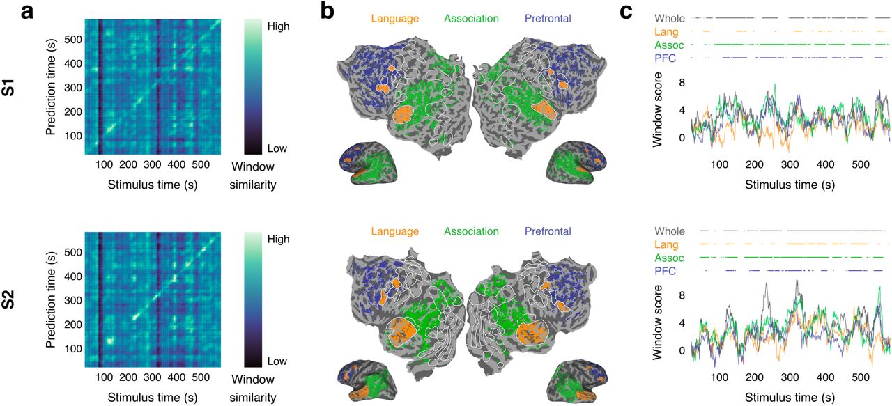
Language decoders were trained for subjects S1 and S2 and then evaluated on single-trial BOLD fMRI responses recorded while the subjects listened to the test story “Where There’s Smoke” by Jenifer Hixson from The Moth Radio Hour. (a) Identification accuracy for whole brain decoder predictions. The brightness at (𝑖, 𝑗) reflects the BERTScore similarity between the 𝑖th second of the decoder prediction and the 𝑗th second of the actual stimulus. Identification accuracy was significantly higher than expected by chance (p < 0.05, one-sided permutation test). (b) Cortical networks for subjects S1 and S2. Brain data used for decoding (colored voxels) were partitioned into the classical language network, the parietal-temporal-occipital association network, and the prefrontal network (PFC). (c) Decoding performance time-course from each network. Horizontal lines indicate when decoder predictions were significantly more similar to the actual stimulus than expected by chance under the BERTScore metric (q(FDR) < 0.05, one-sided nonparametric test). Corresponding results for subject S3 are shown in Figures 1f, 2a, and 2c in the main text.
Supplementary Information
Language decoders were trained for each subject and then evaluated on single-trial BOLD fMRI responses recorded while that subject listened to the test story “Where There’s Smoke” by Jenifer Hixson from The Moth Radio Hour. The actual stimulus words are shown alongside the decoder predictions for each subject. Highlighted segments were significantly more similar to the actual stimulus than expected by chance under the BERTScore metric (q(FDR) < 0.05, one-sided nonparametric test). The decoders recovered the meaning of the perceived story.
Language decoders were trained for each subject (using data collected during story perception) and then evaluated on single-trial BOLD fMRI responses recorded while that subject imagined telling 1-minute segments from five different test stories from Modern Love. The story segments that the subjects were instructed to imagine are shown alongside the decoder predictions for each subject. Highlighted segments were significantly more similar to the reference stimulus than expected by chance under the BERTScore metric (q(FDR) < 0.05, one-sided nonparametric test). Decoder predictions were also significantly similar to transcripts recorded from each subject (q(FDR) < 0.05; not shown). Results are shown for the second repeats of each segment; results for the first repeats were similar. The decoders recovered the meaning of the imagined stories.
Language decoders were trained for each subject (using data collected during story perception) and then evaluated on single-trial BOLD fMRI responses recorded while that subject watched three animated short films from Pixar Animation Studios (“La Luna”, “Presto”, and “Partly Cloudy”) without sound. Reference transcripts—obtained from official audio descriptions for the visually impaired—are shown alongside the decoder predictions for each subject. Highlighted segments were significantly more similar to the reference words than expected by chance under the BERTScore metric (q(FDR) < 0.05, one-sided nonparametric test). The decoders generated language descriptions that capture the meaning of the perceived movies.
Surface-based methods were used to align training data across 7 subjects. Cross-subject decoders were trained for each subject using aligned data from the remaining 6 subjects, and then evaluated on single-trial BOLD fMRI responses recorded while that subject listened to the test story “Where There’s Smoke” by Jenifer Hixson from The Moth Radio Hour. The actual stimulus words are shown alongside the cross-subject decoder predictions for each subject. Highlighted segments were significantly more similar to the stimulus words than expected by chance under the BERTScore metric (q(FDR) < 0.05, one-sided nonparametric test). Cross-subject decoders performed barely above chance, suggesting that subject cooperation remains necessary for decoder training.
Acknowledgements
We thank J. Wang, XX. Wei, and L. Hamilton for comments on the manuscript. This work was supported by the Whitehall Foundation, Alfred P. Sloan Foundation, and the Burroughs Wellcome Fund.
References
Methods References


Subject Area
