Undoubtedly, Natural Language Processing (NLP) research has taken enormous leaps after being relatively stationary for a couple of years. Firstly, Google’s Bidirectional Encoder Representations from Transformer (BERT) [1] becoming the highlight by the end of 2018 for achieving state-of-the-art performance in many NLP tasks and not much later, OpenAI’s GPT-2 stealing the thunder by promising even more astonishing results which reportedly rendering it too dangerous to publish! Considering the time frame and the players behind these publications, it takes no effort to realize that there is a lot of activity in the space at the moment.

That being said, we will focus on BERT for this post and attempt to have a small piece of this pie by extracting pre-trained contextualized word embeddings like ELMo [3].

To give you a brief outline, I will first give a little bit of background context, then a take a high-level overview of BERT’s architecture, and lastly jump into the code while explaining some tricky parts here and there.

Just for more convenience, I will be using Google’s Colab for the coding but the same code can as well run on your local environment without many modifications.

If you came just for the coding part, skip to the “BERT Word Embedding Extraction” section. Find the finished notebook code here.

Word Embeddings

To start off, embeddings are simply (moderately) low dimensional representations of a point in a higher dimensional vector space. In the same manner, word embeddings are dense vector representations of words in lower dimensional space. The first, word embedding model utilizing neural networks was published in 2013 [4] by research at Google. Since then, word embeddings are encountered in almost every NLP model used in practice today. Of course, the reason for such mass adoption is quite frankly their effectiveness. By translating a word to an embedding it becomes possible to model the semantic importance of a word in a numeric form and thus perform mathematical operations on it. To make this more clear I will give you the most common example that you can find in the context of word embeddings

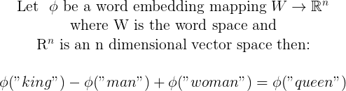
When this was first possible by the word2vec model it was an amazing breakthrough. From there, many more advanced models surfaced which not only captured a static semantic meaning but also a contextualized meaning. For instance, consider the two sentences below:

I like apples.

I like Apple macbooks

Note that the word apple has a different semantic meaning in each sentence. Now with a contextualized language model, the embedding of the word apple would have a different vector representation which makes it even more powerful for NLP tasks.

However, I will leave the details of how that works, out of the scope of this post just to keep it short and on point.

Transformers

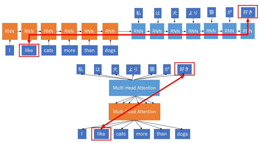
To be frank, much of the progress in the NLP space can be attributed to the advancements of general deep learning research. More particularly, Google (again!) presented a novel neural network architecture called a transformer in a seminal paper [5] which had many benefits over the conventional sequential models (LSTM, RNN, GRU etc). Advantages included but were not limited to, the more effective modeling of long term dependencies among tokens in a temporal sequence, and the more efficient training of the model in general by eliminating the sequential dependency on previous tokens.

In a nutshell, a transformer is an encoder-decoder architecture model which uses attention mechanisms to forward a more complete picture of the whole sequence to the decoder at once rather than sequentially as illustrated in the figures below.

Again, I won’t be describing details about how attention works as it will make the topic way more confusing and harder to digest. Feel free to follow the relevant paper in the references.

OpenAI’s GPT was the first to create a transformer based language model with fine tuning but to be more precise, it was only using the decoder of the transformer. Therefore, making the language modeling uni-directional. The technical reason for dropping out the encoder was that language modeling would become a trivial task as the word to be predicted could have ultimately seen itself.

Bidirectional Encoder Representations from Transformer (BERT)

By now, the name of the model should probably make more sense and give you a rough idea of what it is. BERT brought everything together to build a bidirectional transformer-based language model using encoders rather than decoders! To overcome the “see itself” issue, the guys at Google had an ingenious idea. They employed masked language modeling. In other words, they hid 15% of the words and used their position information to infer them. Finally, they also mixed it up a little bit to make the learning process more effective.

Although this methodology had a negative impact on convergence time, it outperformed state-of-the-art models even before convergence which sealed the success of the model.

Normally, BERT represents a general language modeling which supports transfer learning and fine-tuning on specific tasks, however, in this post we will only touch the feature extraction side of BERT by just obtaining ELMo-like word embeddings from it, using Keras and TensorFlow.

But hold your horses! Before we jump into the code let’s explore BERT’s architecture really quick so that we have a bit of background at implementation time. Believe me, it will make things a lot easier to understand.

In fact, BERT developers created two main models:

1. The BASE: Number of transformer blocks (L): 12, Hidden layer size (H): 768 and Attention heads(A): 12
2. The LARGE: Number of transformer blocks (L): 24, Hidden layer size (H): 1024 and Attention heads(A): 16

In this post, I will be using the BASE model as it is more than enough ( and way smaller!).

From a very high-level perspective, BERT’s architecture looks like this:

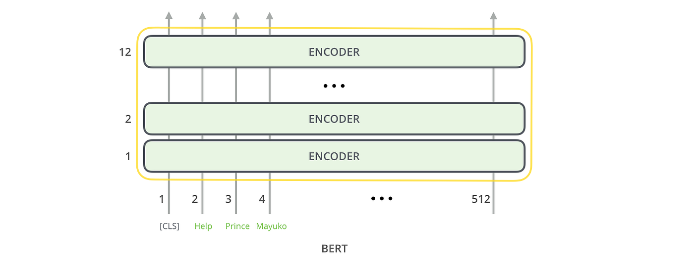
It may seem simple but remember that each encoder block encapsulates a more sophisticated model architecture.

At this point, to make things clearer it is important to understand the special tokens that BERT authors used for fine-tuning and specific task training. These are the following:

1. [CLS] : The first token of every sequence. A classification token which is normally used in conjunction with a softmax layer for classification tasks. For anything else, it can be safely ignored.
2. [SEP] : A sequence delimiter token which was used at pre-training for sequence-pair tasks (i.e. Next sentence prediction). Must be used when sequence pair tasks are required. When a single sequence is used it is just appended at the end.
3. [MASK] : Token used for masked words. Only used for pre-training.

Moving on, the input format that BERT expects is illustrated below:

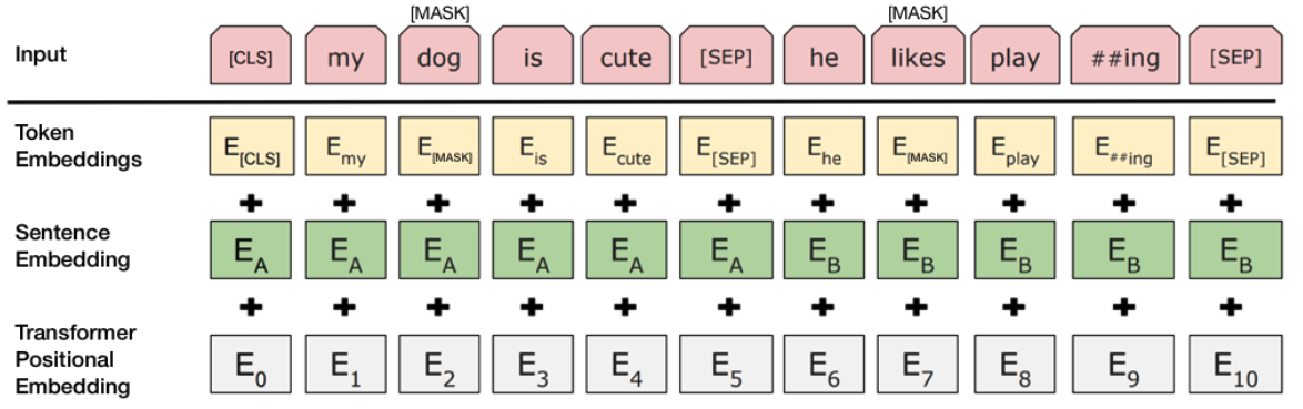
As such, any input to be used with BERT must be formatted to match the above.

The input layer is simply the vector of the sequence tokens along with the special tokens. The “##ing” token in the example above may raise some eyebrows so to clarify, BERT utilizes WordPiece [6] for tokenization which in effect, splits token like “playing” to “play” and “##ing”. This is mainly to cover a wider spectrum of Out-Of-Vocabulary (OOV) words.

Token embeddings are the vocabulary IDs for each of the tokens.

Sentence Embeddings is just a numeric class to distinguish between sentence A and B.

And lastly, Transformer positional embeddings indicate the position of each word in the sequence. More details on this one can be found in [5].

Finally, there is one last thing. Everything is great is sofar, but how can I get word embeddings from this?!? As discussed, BERT base model uses 12 layers of transformer encoders, each output per token from each layer of these can be used as a word embedding! You probably wonder, which one is the best though? Well, I guess this depends on the task but empirically, the authors identified that one of the best performing choices was to sum the last 4 layers, which is what we will be doing.

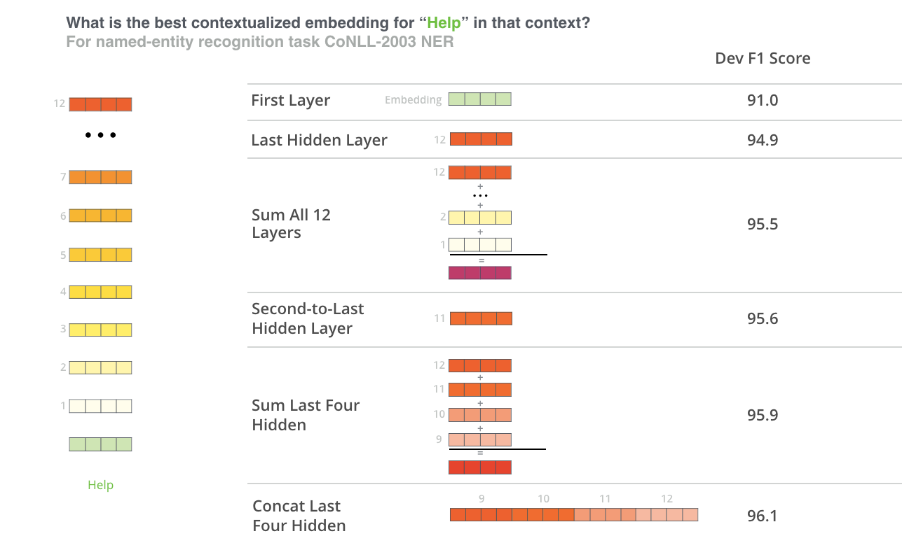
As illustrated the best performing option is to concatenate the last 4 layers but in this post, the summing approach is used for convenience. More particularly, the performance difference is not that much, and also there is more flexibility for truncating the dimensions further, without losing much information.

BERT Word Embedding Extraction

Enough with the theory. Let’s move on to the practice.

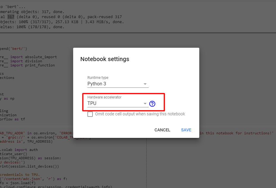
Firstly, create a new Google Colab notebook. Go to Edit->Notebook Settings and make sure hardware accelerator is set to TPU.

Now, the first task is to clone the official BERT repository, add its directory to the path and import the appropriate modules from there.

!rm -rf bert
!git clone https://github.com/google-research/bertimport syssys.path.append('bert/')from __future__ import absolute_import
from __future__ import division
from __future__ import print_functionimport codecs
import collections
import json
import re
import os
import pprint
import numpy as np
import tensorflow as tfimport modeling
import tokenization

The two modules imported from BERT are modeling and tokenization. Modeling includes the BERT model implementation and tokenization is obviously for tokenizing the sequences.

Adding to this, we fetch our TPU address from colab and initialize a new tensorflow session. (Note that this only applies for Colab. When running locally, it is not needed). If you see any errors on when running the block below make sure you are using a TPU as hardware accelerator (see above)

Moving on, we select which BERT model we want to use.

As you can see there are three available models that we can choose, but in reality, there are even more pre-trained models available for download in the official BERT GitHub repository. Those are just the models that have already been downloaded and hosted by Google in an open bucket so that can be accessed from Colaboratory. (For local use you need to download and extract a pre-trained model).

Recall the parameters from before: 12 L (transformer blocks) 768 H (hidden layer size) 12 A (attention heads) . “Uncased” is just for lowercase sequences. In this example, we will use the uncased BERT BASE model.

Furthermore, we define some global parameters for the model:

Most of the parameters above are pretty self-explanatory. In my opinion, the only one that may be a little bit tricky is the LAYERS array. Recall that we are using on the last 4 layers from the 12 hidden encoders. Hence, LAYERS keeps their indices.

The next part is solely to define wrapper classes for the input before processing and after processing (Features).

In the InputExample class, we have set text_b to None by default since we aim to use single sequences rather than a sequence-pairs.

Moreover, the InputFeatures class encapsulates the features that BERT needs for input (See input diagram above). The tokens property is clearly a vector of input tokens, input_ids are the ids that correspond to the token from the vocabulary, input_mask annotates real token sequence from padding and lastly, input_type_ids separates segment A from segment B so it is not really relevant here.

Now, add the following code:

This is to set up our Estimator. An Estimator is just an abstraction for a model that tensorflow provides along with an API for training, evaluation, and prediction. Our custom estimator is, therefore, a wrapper around the BertModel. Admittedly there are parts of the code that can be removed from the above but I am sticking to the example that Google provided just for consistency. The important parts there is line 60 — where the bert model is defined — , and line 100 where the predictions from the top 4 layers are extracted.

Continue along by also adding the following:

This is the function that takes care of the input processing. In other words, it transforms InputExamples to InputFeatures.

Adding to these, we create a function for converting a normal string sequence to InputExample:

Now for the last bit of the code, we define a function which accepts an array of strings as a parameter and the desired dimension (max 768) of the embedding output and returns a dictionary with the token as key and the embedding vector as value.

The above code snippet simply builds the estimator and invokes a prediction based on the given inputs.

Let’s go ahead and test our model by running this:

embeddings = get_features([“This is a test sentence”], dim=50)
print(embeddings)

If everything goes well, you will have a dictionary containing the embeddings of size 50 per token. Remember that these are contextualized embeddings, so if you have duplicate tokens on different sequences only the embedding of the last token will be kept in the dictionary. To keep both, replace the dictionary with a different data structure.

You can find the complete notebook here.

Future Work

Now, these embeddings can be used as input features for other models built for custom tasks. Nevertheless, I will save that for another post. Or even maybe implement a BERT Keras Layer for seamless embedding integration.

Conclusion

That’s all from me folks. I hope you enjoyed the post and hopefully got a clearer picture around BERT. Feel free to post your feedback or questions in the comments section.

References:

[1] J.Devlin, M. Chang, K. Lee and K. Toutanova, BERT: Pre-training of Deep Bidirectional Transformers for Language Understanding (2018)

[2] Radford, Alec, Wu, Jeff, Child, Rewon, Luan, David, Amodei, Dario, Sutskever, Ilya, Language Models are Unsupervised Multitask Learners (2019)

[3] M. Peters, M. Neumann, M. Iyyer, M. Gardner, C. Clark, K.Lee and L.Zettlemoyer, Deep contextualized word representations (2018), North American Chapter of the Association for Computational Linguistics

[4] T.Mikolov, I. Sutskever, K. Chen, G. Corrado and J. Dean, Distributed Representations of Words and Phrases and their Compositionality (2013)

[5]A. Vaswani, N. Shazeer, N. Parmar, J. Uszkoreit, L. Jones, A.Gomez, L. Kaiser and I. Polosukhin, Attention Is All You Need (2017)

[6] Y. Wu, M. Schuster, Z. Chen, Q. Le, M. Norouzi, W. Macherey, M. Krikun, Y. Cao, Q. Gao, K. Macherey, J. Klingner, A. Shah, M. Johnson, X. Liu, Ł. Kaiser, S. Gouws, Y. Kato, T. Kudo, H. Kazawa, K. Stevens, G. Kurian, N. Patil, W. Wang, C. Young, J. Smith, J. Riesa, A. Rudnick, O. Vinyals, G. Corrado, M. Hughes and J. Dean Google’s Neural Machine Translation System: Bridging the Gap between Human and Machine Translation (2016)