Explain Your Model with LIME

Dr. Dataman

Follow

Feb 25, 2020 · 7 min read

Why Is Model Interpretability so Important?

Machine learning is great in prediction accuracy, process efficiency, and research productivity. But computers usually do not explain their predictions. This becomes a barrier to the adoption of machine learning models. If the users do not trust a model or a prediction, they will not use or deploy it. Therefore the issue is how to help users to trust a model.

There are several great solutions including SHAP, LIME, and ELI5. In this article I will walk you through the origin of LIME, and how to apply to your analysis. I have also written “Explain Your Model with the SHAP Values”, “Explain Any Models with the SHAP Values — Use the KernelExplainer”, “The SHAP with More Elegant Charts” and “Creating Waterfall Plots for the SHAP Values for All Models”. You can bookmark the summary post “Dataman Learning Paths — Build Your Skills, Drive Your Career” that lists the links to all articles.

“Why Should I Trust You?”

In the seminar work “Why Should I Trust You?” Explaining the Predictions of Any Classifier (KDD2016) by Marco Tulio Ribeiro, Sameer Singh, and Carlos Guestrin, the interpretability for a black-box model has a novel solution. The solution aim at building two types of trust:

• Trusting a prediction: a user will trust an individual prediction to act upon. No user wants to accept a model prediction on blind faith, especially if the consequences can be catastrophic.
• Trusting a model: the user gains enough trust that the model will behave in reasonable ways when deployed. Although in the modeling stage accuracy metrics (such as AUC — Area under the curve) are used on multiple validation datasets to mimic the real-world data, there often exist significant differences in the real-world data. Besides using the accuracy metrics, we need to test the individual prediction explanations.

They proposed a novel technique called the Local Interpretable Model-Agnostic Explanations (LIME). that can explain the predictions of any classifier in “an interpretable and faithful manner, by learning an interpretable model locally around the prediction.” Their approach is to gain the trust of users for individual predictions and then to trust the model as a whole.

What Is “Easily Interpretable”?

People may say that a linear model is easier than a complicated machine learning model. Is it true? The authors of LIME have two criteria:

• Easy to interpret: A linear model can have hundreds or thousands of variables. Is it more interpretable than a complex gradient boosting or deep learning model?
• Local fidelity: the explanation for individual predictions should at least be locally faithful, i.e. it must correspond to how the model behaves in the vicinity of the individual observation being predicted. The authors address that local fidelity does not imply global fidelity: features that are globally important may not be important in the local context, and vice versa. Because of this, it could be the case that only a handful of variables directly relate to a local (individual) prediction, even if a model has hundreds of variables globally.

A model should be easily interpretable. Often we have this impression that a linear model is more interpretable than a ML model. Is it true? Look at this linear model with forty variables. Is it easy to explain? Not really.

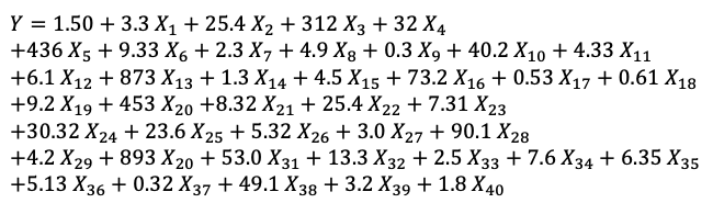
Although this model has forty variables, for an individual prediction there may be only a few variables influencing its predicted value. The interpretation should make sense from an individual prediction’s view. The authors of LIME call this local fidelity. Features that are globally important may not be important in the local context, and vice versa. Because of this, it could be the case that only a handful of variables directly relate to a local (individual) prediction, even if a model has hundreds of variables globally.

That’s why they named this technique Local Interpretable Model-Agnostic Explanations (LIME) — It should be locally interpretable and able to explain any models.

Model Interpretability Does Not Mean Causality

It is important to point out LIME does not provide causality. In the “identify causality” series of articles, I demonstrate econometric techniques that identify causality. Those articles cover the following techniques: Regression Discontinuity (see “Identify Causality by Regression Discontinuity”), Difference in differences (DiD)(see “Identify Causality by Difference in Differences”), Fixed-effects Models (See “Identify Causality by Fixed-Effects Models”), and Randomized Controlled Trial with Factorial Design (see “Design of Experiments for Your Change Management”).

How Is LIME Different from SHAP?

In “Explain Your Model with the SHAP Values” I describe extensively how the SHAP (SHapley Additive exPlanations) is distinctly built on the Shapley value. The Shapley value is the average of the marginal contributions across all permutations. The Shapley values consider all possible permutations, thus SHAP is a united approach that provides global and local consistency and interpretability. However, its cost is time — it has to compute all permutations in order to give the results. In contrast, LIME (Local Interpretable Model-agnostic Explanations) builds sparse linear models around an individual prediction in its local vicinity. This is documented in Lundberg and Lee (2016) that LIME is actually a subset of SHAP but lacks the same properties.

The Advantage of LIME over SHAP — SPEED

Readers may ask: “If SHAP is already a united solution, why should we consider LIME?” Remember, the two methods emerge very differently. The advantage of LIME is speed. LIME perturbs data around an individual prediction to build a model, while SHAP has to compute all permutations globally to get local accuracy. Further, the SHAP Python module does not yet have specifically optimized algorithms for all types of algorithms (such as KNNs), as I have documented in “Explain Any Models with the SHAP Values — Use the KernelExplainer” that test models in KNN, SVM, Random Forest, GBM, or the H2O module.

How Does LIME Work?

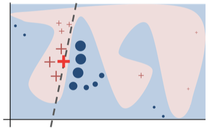
The authors of LIME have an intuitive graph as shown in Figure (A). The original complex model is represented by the blue/pink background. It is obviously not linear. The bold red cross is the individual prediction to be explained. The algorithm of LIME does the following steps:

• Generating new samples then gets their predictions using the original model, and
• Weighing these new samples by the proximity to the instance being explained (represented in Figure (A) by size).

Then it builds a linear regression for these newly created samples including the red cross. The dashed line is the learned explanation that is locally (but not globally) faithful.

How to Use LIME in Python?

In order to let you compare SHAP and LIME, I use the red wine quality data used in “Explain Your Model with the SHAP Values” and “Explain Any Models with the SHAP Values — Use the KernelExplainer”. The target value of this dataset is the quality rating from low to high (0–10). The input variables are the content of each wine sample including fixed acidity, volatile acidity, citric acid, residual sugar, chlorides, free sulfur dioxide, total sulfur dioxide, density, pH, sulphates and alcohol. There are 1,599 wine samples. You can get the code via this github. The following code builds a random forest model:

I am going to apply the model to the first two records of the test data X_test. The Y values of the two records are ‘6’ and ‘5’ (you can obtain them byY_test[0:2]), and the predictions are 5.58, 4.49 respectively (use model.predict(X_test[0:2])).

You will install the LIME module from this Github. The code below builds the LIME model explainer.

Why is it named “lime_tabular”? LIME names it for tabular (matrix) data, in contrast to “lime_text” for text data and “lime_image” for image data. In our example all predictors are numeric. LIME perturbs the data by sampling from a Normal(0,1) and doing the inverse operation of mean-centering and scaling, according to the means and standard deviations in the training data. If you have categorical variables, LIME perturbs the data by sampling according to the training distribution, and creates a binary feature of 1 if the value is the same as the instance being explained.

(A) Interpret the first record:

You can create a plot for each individual. Use num_features to specify the number of features displayed.

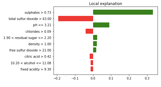
• Green/Red color: features that have positive correlations with the target are shown in green, otherwise red.
• Sulphates>0.73: high sulphate values positively correlate with high wine quality.
• Total sulfur dioxide>63.0: high total sulfur dioxide values negatively correlate with high wine quality.
• ph≤3.21: low ph values positively correlate with high wine quality.
• Use the same logic to understand the rest features.

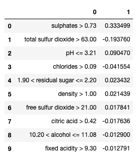
You can obtain the coefficients of the LIME model by as_list():

And you can show all the results in a notebook-like format:

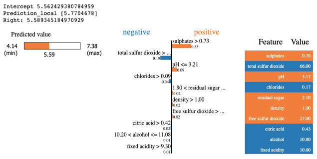
• The LIME model intercept: 5.562,
• The LIME model prediction: “Prediction_local 5.770”, and
• The original random forest model prediction: “Right: 5.589”.

How does LIME get its Prediction_local 5.770? It is the intercept plus the sum of the coefficients. Because the intercept is 5.562 and the total of the coefficients is 0.208 (obtained by pd.DataFrame(exp.as_list())[1].sum()), the LIME prediction is 5.678 + 0.208 = 5.770.

(B) Interpret the second record:

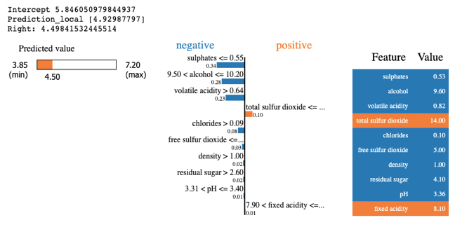
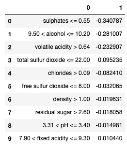
The sum of the above coefficients is -0.916. Because the intercept is 5.846, the LIME prediction becomes 5.846 -0.916 = 4.929.