Equalizing Headphones the Easy Way

Jaakko Pasanen

Feb 17, 2019·9 min read

Driven by advancements in active noise cancelling and wireless technologies popularity of over ear headphones has increased rapidly in recent years. Now convenience and looks are considered to be the most important attributes for many when selecting a pair to buy. Consumers are not usually knowledgeable enough in audio to prioritize sound quality giving manufacturers and incentive to focus on other things and manufacturers might even go as far as tune the sound of headphones deliberately “bad” by for example increasing bass to unnaturally high level to induce an excited reaction in potential buyers. However this can be largely fixed and this article show’s you how to do it.

Sound quality of a headphone is mostly determined by it’s frequency response. Frequency response describes the balance of different frequencies: bass, mid and treble. Headphones are going to sound unnatural if the their frequency response doesn’t match how humans perceive sound coming from speakers in a room. Music is recorded, mixed and mastered to be listened with speakers so headphones should try to imitate that experience.

Unexpected and unfortunate reality is that more expensive headphones don’t have any better frequency responses than cheaper ones. This means you cannot simply buy an expensive headphone and trust that you get a good sounding one. Fortunately you don’t have to buy expensive headphones because even affordable ones can be made to sound good by equalizing the frequency response to match the natural one. In matter of a fact a $100 headphone equalized to sound natural will be preferred by most people to many high end headphones costing thousands of dollars when not equalized. Turning the knobs and sliders yourself without having a lot of practice in this often leaves you worse, not better, but there is an easier way…

Introducing AutoEQ

AutoEQ (https://github.com/jaakkopasanen/AutoEq) is a tool for equalizing headphones to sound more natural, better. While the project has many benefits for developers and technical people the main attraction for most is the pre-computed equalizer settings for over 1400 headphone models. Simply head to the results section, search for you headphone model and follow the usage instructions.

AutoEQ itself doesn’t do the live equalization but produces settings which can be used in various equalizer apps. AutoEQ’s pre-computed results include parametric equalizer parameters, standard 10 band graphical equalizer levels and impulse responses for convolution based equalizers. These all mean that basically all platforms and devices are covered.

Add Your Own

You can create equalization settings for your own headphone if that model cannot be found in the pre-computed results and you have the frequency response graph available. Frequency response graphs come in many outfits and can be found all around the web with a little bit of Googling although not all of the headphones ever produced have been measured. Frequency response graphs look like these:

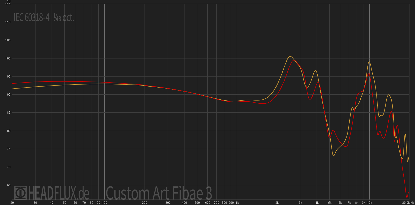
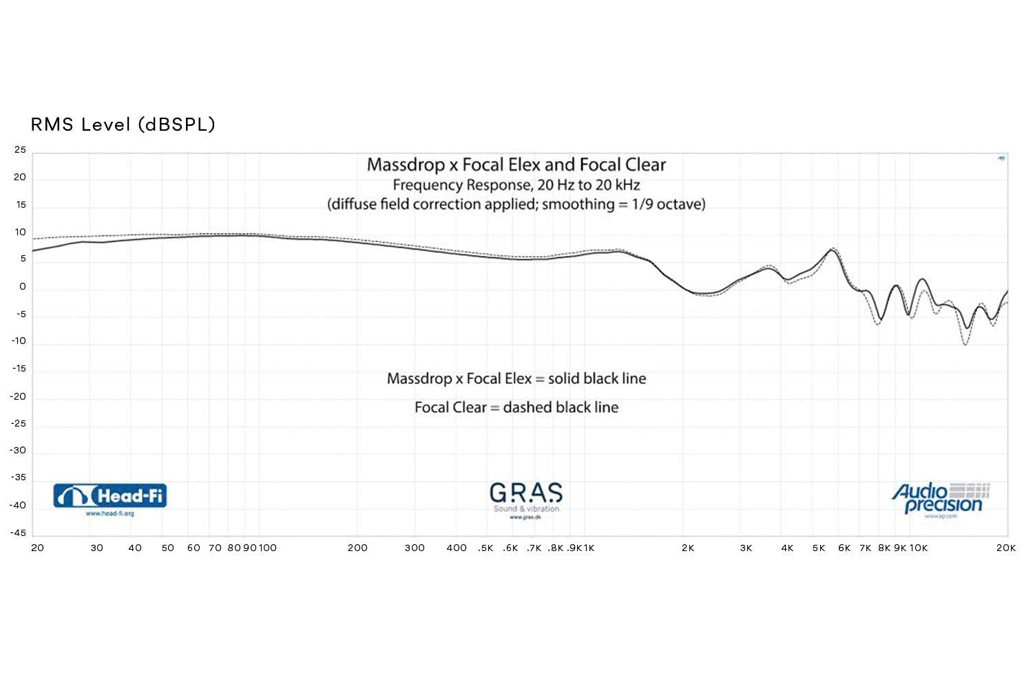
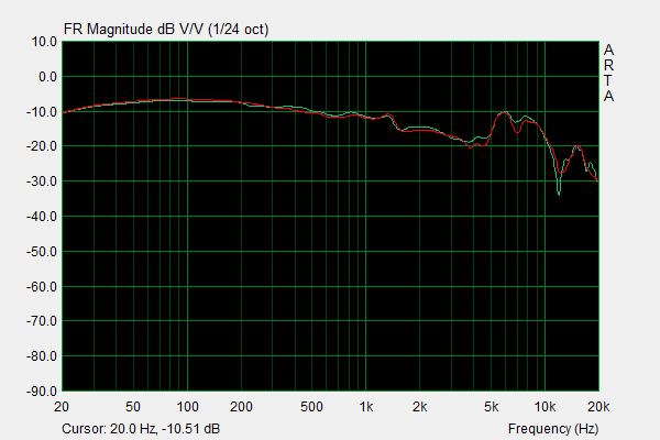
Some graphs are raw frequency responses measured by the microphone and some are compensated with a target frequency response. Compensated ones are actually not frequency responses strictly speaking but deviations (errors) from the natural frequency response. Compensated measurements vary wildly with the used compensation and not all measurement system and compensation curves are created equal.

The first of the three graphs above is not compensated so a compensation is required when creating equalization settings. Measurement system used for this measurement happens to be compatible with the latest research by Harman international so it’s possible to use any of the Harman in-ear targets for compensation. When dealing with uncompensated graphs you essentially have to know which compensation curve to use or just try out for example latest Harman target and hope for the best.

The middle one has been compensated with diffuse field response and therefore can be used with zero compensation. Many people consider diffuse field too bright, to have too much treble, so using that might not produce ideal results. The last graph looks to be compensated but compensation curve is not disclosed. This is often the case although you can try to investigate if you can find a mention about the compensation curve. In any case we have to deal with what we have and ideal results cannot be expected every time when using random frequency response graphs.

The right most graph doesn’t say that it’s compensated and knowing might be difficult in these cases. Headphones should have a peak at 3 kHz of about 10 to 15 dB so if that peak is there in the graph then it’s most likely is not compensated. Some headphones deviate a lot from the ideal target and in these cases equalizing with and without compensation and listening which is better might be the only way to know.

Numbers From the Graph

AutoEQ requires input data to be numeric CSV file so the numerical values need to be read from the graph image. WebPlotDigitizer comes to aid here. With WebPlotDigitizer you can load the image, set graph axis alignments and set parameters for finding the curve pixels. Here’s how.

First go to https://apps.automeris.io/wpd/ and load you image with “Load Image” button.

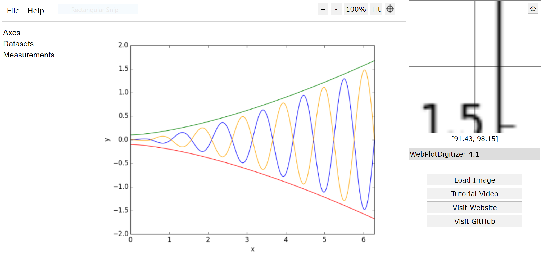
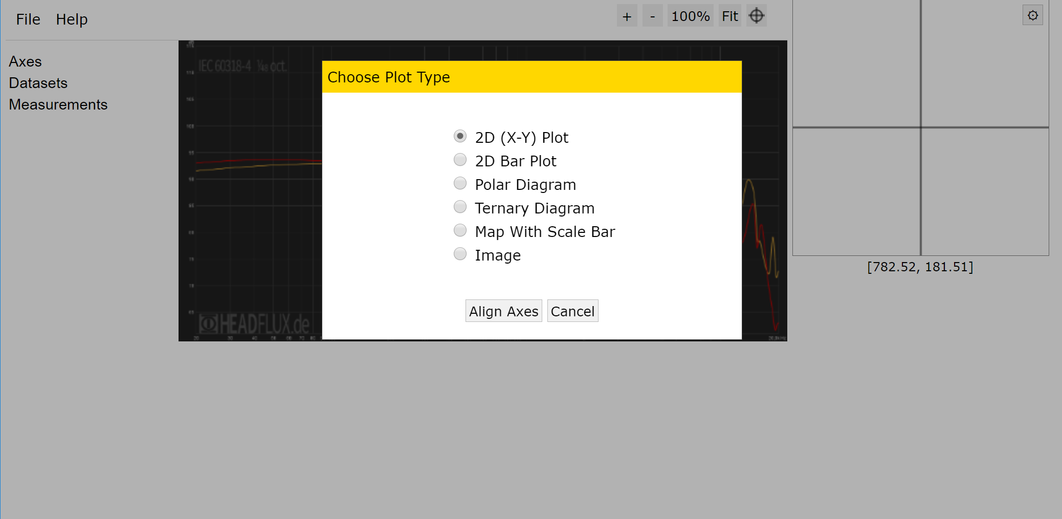
Choose “2D (X-Y) Plot” as the plot type and click “Align Axes”.

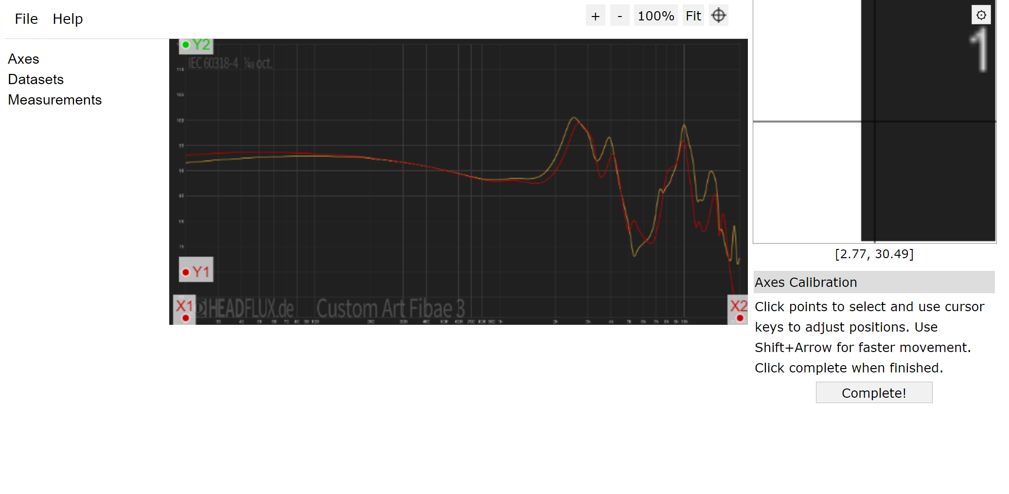
Align axes by clicking the image with cursor. First on the X-axis at 20 Hz and then on the X-axis at 20 kHz. Do the same for Y-axis and select lowest and highest points in Y-axis which have a number next to them. Both points on X-axis must be on the same vertical level and both points on Y-axis must be on the same horizontal level. Zoom window on the top right corner shows you more accurate view. When you have all four points set click “Complete”.

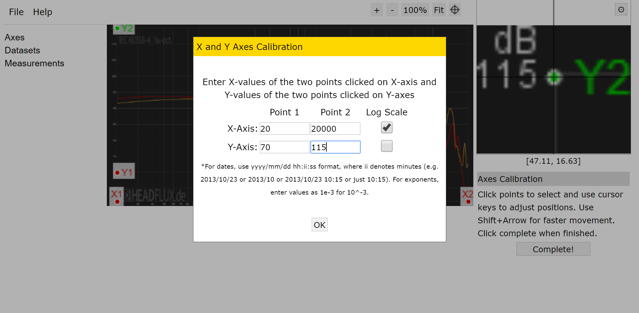
Set values for X and Y-axis. Zoom window on the top will show the vicinity of the clicked point when selecting respective input field. You should see the number label if you clicked all the points on axes near labels. When all values are in the input fields select “Log Scale” for X-axis. Click “OK” to finish.

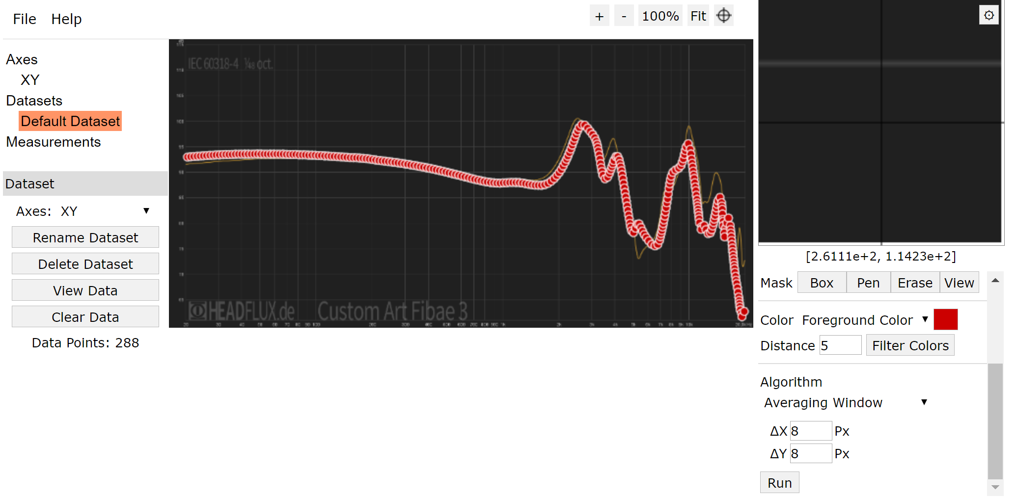
After axes have been aligned and scaled you need to set parameters for reading the graph pixels from the image. Set foreground color to the curve color by clicking the colored square next to “Foreground Color” and use “Color Picker” to pick a color from the curve. Make sure to click right in the middle of the line for best results. Set “Distance” to a low value like 5 and set smaller “Averaging Window” values if your image resolution is low. Click “Run” to find curve points.

If there are curve points missing try increasing color distance or picking a new color. If there are evenly spaced points but they are too few or too many try adjusting averaging window size. If the image has same colored pixels outside of the curve you can use “Box” or “Pen” tools to mark the curve area and the WebPlotDigitizer will know to ignore other pixels.

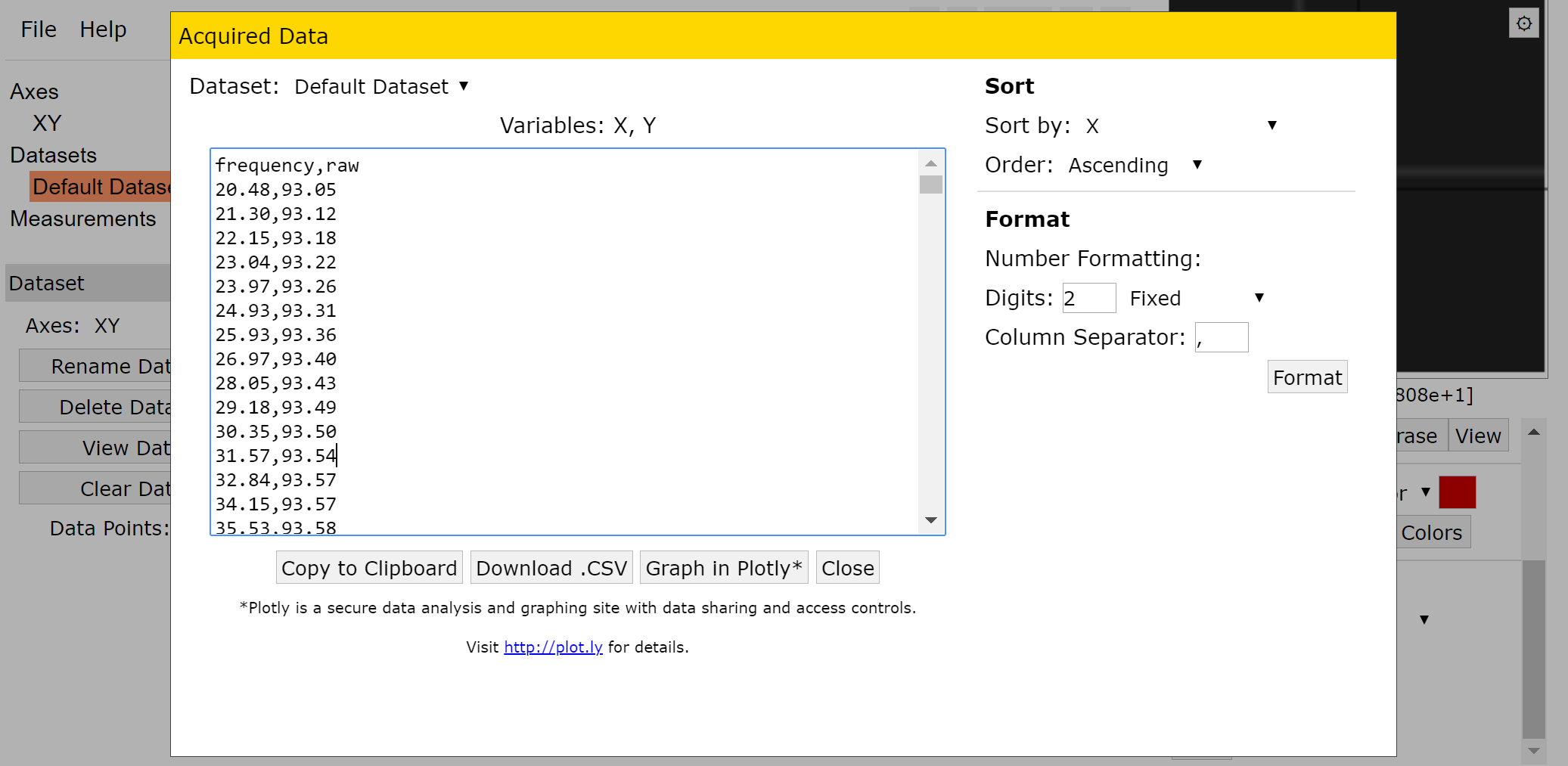
Click “View Data” on the left hand side to open data view dialog. Here set “Sort By:” to “X” and “Order” to “Ascending”. Set “Digits” to 2 “Fixed” and remove the space after comma in the “Column Separator”. The column separator input field should have “,” instead of “, “. Click “Format” to format the data. Finally add header row “frequency,raw” as the first line in the data text area. In this stage it’s a good idea to check that there are no lines with duplicate frequency values. AutoEQ will inform about these but things will go more smoothly if you just remove them now.

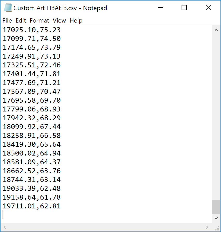
Copy-paste the text data into a text editor like Notepad and save the file with headphone model name with “.csv” file extension. In this example the file is going to be “Custom Art FIBAE 3.csv”. If you are using Notepad set encoding to UTF-8 and file type to “All files” when saving. If you have, or are willing to install, some better text editor like Notepad++ you should use that because in some cases Notepad might do nasty things to character encoding.

Using AutoEQ

Once you have the CSV file created it’s time to fire up AutoEQ. Start by visiting https://github.com/jaakkopasanen/AutoEq and clicking the green “Clone or download” button on top right. Use git clone if you’re familiar with Git and “Download ZIP” if you’re not. Exctract the zip to convenient location, open up a terminal (command prompt) and navigate to the extracted location. Follow installing instructions and try out some example commands to get going.

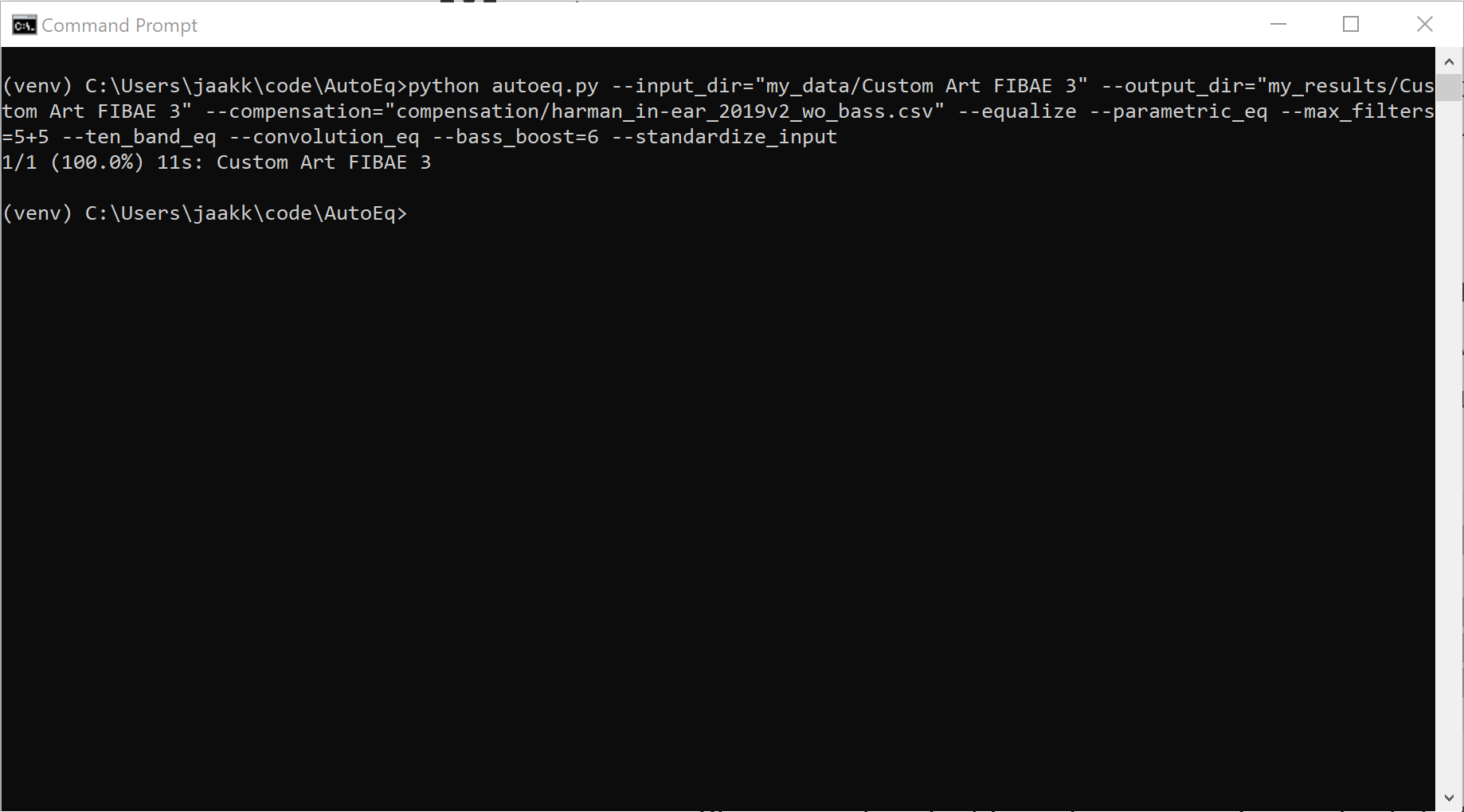
You got AutoEq installed and working so the next thing is to create equalization settings from the CSV file you created with WebPlotDigitizer. Move the file into “AutoEq/my_data/Custom Art FIBAE 3/Custom Art FIBAE 3.csv” (or what ever your headphone model is) and run:

python autoeq.py --input_dir="my_data/Custom Art FIBAE 3" --output_dir="my_results/Custom Art FIBAE 3" --compensation="compensation/harman_in-ear_2019v2_wo_bass.csv" --equalize --parametric_eq --max_filters=5+5 --ten_band_eq --convolution_eq --bass_boost=6 --standardize_input

Your results can be found in “AutoEq/my_results” folder. Parametric eq filters and such can be found in the README.md file. Fire up your equalizer of choice, configure settings and enjoy audio nirvana.

Here are the example result graphs.

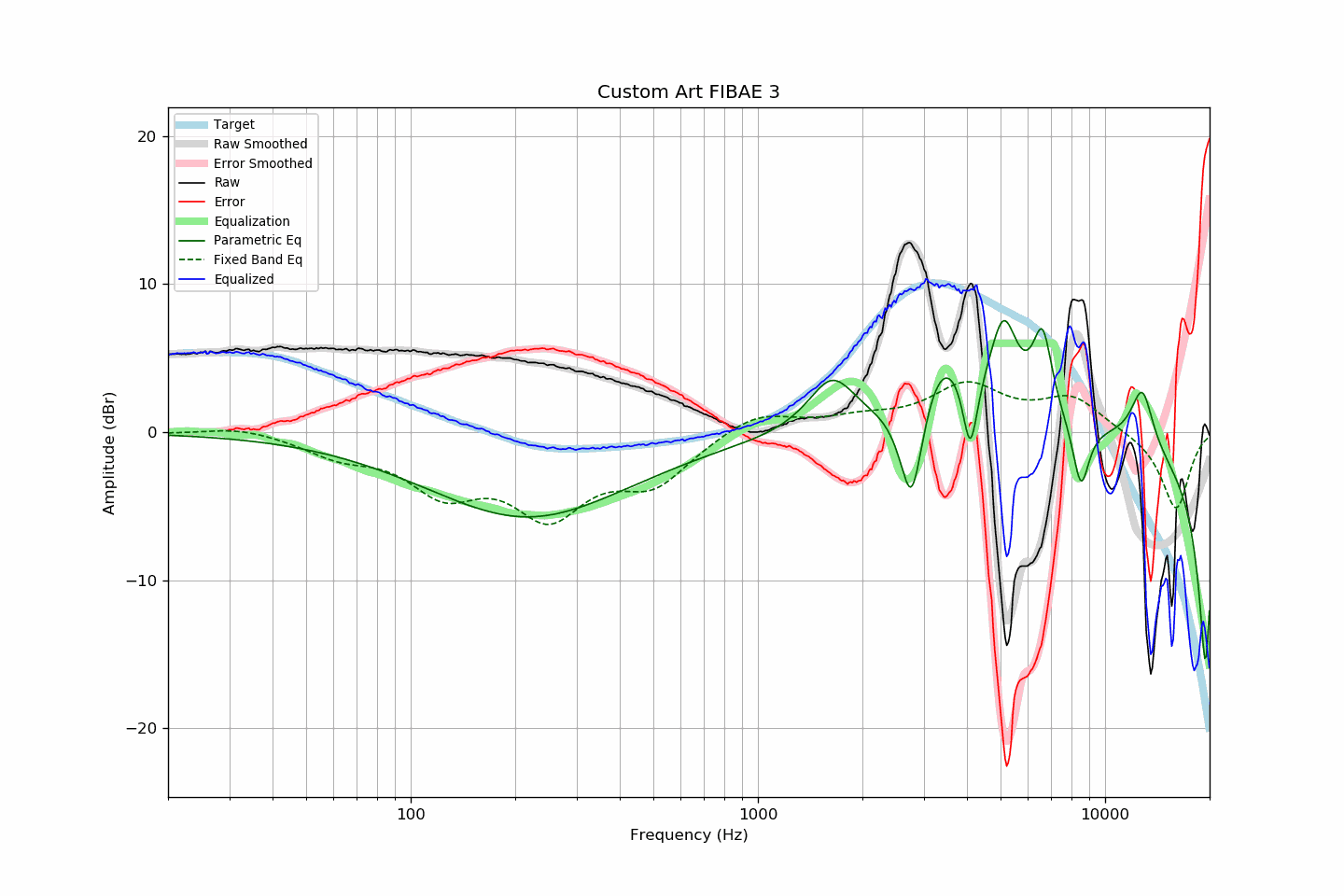
The measurement used in this example is made with a measurement system that is compatible with Harman in-ear targets so that is what is used as the compensation curve with --compensation parameter. Note that the selected compensation file “harman_in-ear_2019v2_wo_bass.csv” doesn’t have a bass boost because we added the bass boost with AutoEq. Preferred bass boost levels differ greatly from person to person so it’s better to adjust it to your liking.

When dealing with graphs that are already compensated you need to supply flat curve as the compensation file. This can be done with
--compensation="compensation/zero.csv" .

Results have 10 parametric equalizer filters optimized of which first 5 can be used independently. You can adjust this with --max_filters parameter if needed. --ten_band_eq parameter activates optimization for standard 10 band graphic equalizer. --bass_boost=6 sets bass boost shelf to +6dB. Finally --standardize_input causes the input file to be updated to AutoEQ standard format.

There are several other parameters which you can use to fine tune the result and you can read more about those in the command line arguments documentation.

Thanks for reading!

If you have problems with this guide or have ideas how to do things better comment in Issue 22.

References

https://asa.scitation.org/doi/abs/10.1121/1.4984044