


前置きというか概要
今年のEMNLP2017で提案されていたSCDV(Sparse Composite Document Vectors)について、日本語のコーパス()で検証しました。
SCDVのモチベーション
(https://dheeraj7596.github.io/SDV/)
いい感じのランディングページまで用意していてすげえなって思いました。論文は当然のようにarxivで公開されています。大正義。
https://arxiv.org/pdf/1612.06778.pdf
HTMLで読みたい方はこちら。https://www.arxiv-vanity.com/papers/1612.06778/
これを読んでいる皆様に、「どうにかして文章のベクトルが欲しいんです!単語じゃないんです!お願いします!なんでもしますから!」という依頼が来たら、どんな感じで対処しますでしょうか。
doc2vecでしょうか。それともdoc2vecは精度があんまりよくないから基本に忠実にTFIDFでしょうか。もしやなのですが、何か学習済みWord2Vecのモデルを使って、ある文章中に現れる単語のベクトルを足し上げて最後に平均することでその文章のベクトルとしていたりしないでしょうか。
わざとらしい感じに持って行ってしまいましたが、SCDVはそんな風に、単語ベクトルの平均で文書ベクトルを作る際の精度向上を目的とした提案手法です。
SCDVは何をする手法なのか
では、SCDVはどのようにしてそれを実現するのかといいますと、word2vecのベクトル空間をいい感じに修正することがその本質です。
より具体的に言うと、word2vecのベクトル空間をクラスタリングして、各単語がどのトピックに属しているのか、それを考慮したベクトル空間に修正してあげようと言う感じです。アルゴリズム自体はめちゃくちゃ単純で、以下の通り。
- ある単語のベクトルを取得(word2vec)
- ある単語のIDF値を計算する
- GMM(ソフトクラスタリング)で全単語ベクトルについてクラスタリングを行い、ある単語が各クラスタに属する確率を取得する
- 語彙空間における各単語について5を繰り返す
- 各クラスタについてクラスタの数だけ6を繰り返す。クラスタの数だけ計算したら、7を実行する
- クラスタを考慮した新たな単語ベクトルをとして算出
- IDFを考慮した新たな単語ベクトルをで算出(はconcatenation)
- 各ドキュメント()について9の操作を繰り返す
- ドキュメントについてベクトルを初期化し、に含まれる単語についてベクトルを足し合わせていき平均する
- 最後に得られた文書ベクトルをスパースにしてを得る
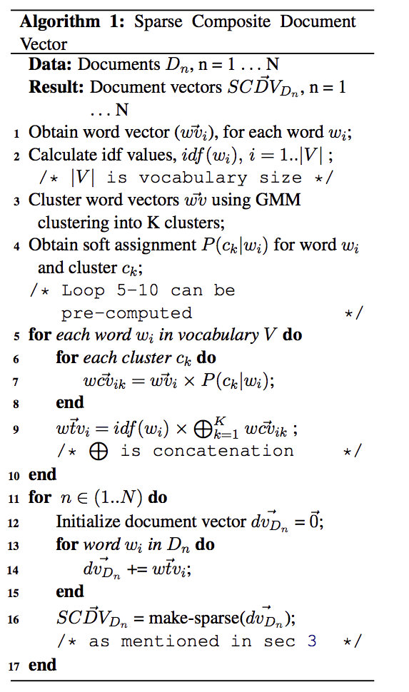
7までで修正した単語ベクトル表現が手に入り、8,9,10で各ドキュメントのベクトルが手に入ります。
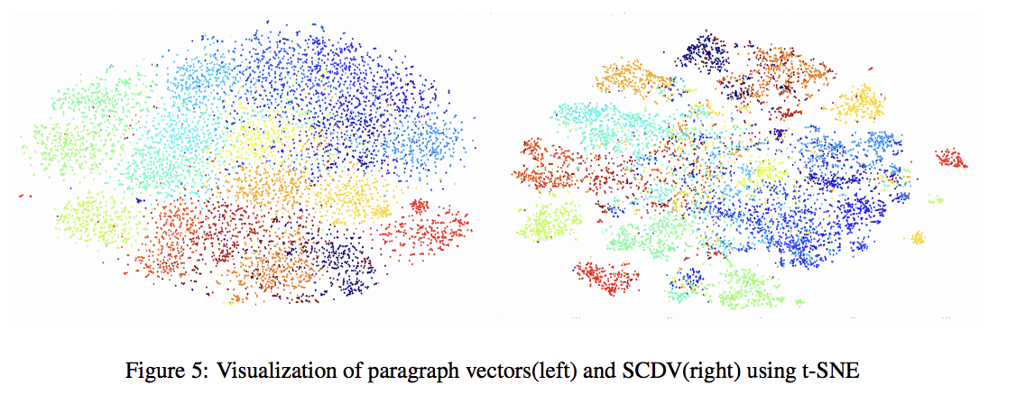
tsneで文書ベクトルを可視化するとこんな感じになるんだそう。左がプレーンで右がSCDVです。確かに良くなっているように見える。各クラスタがはっきりしているように見えます。
で、これで文書分類タスクをやってみたら、既存の文書ベクトル表現よりも精度が良かったよ、というらしいのです。ほんとか〜〜〜?
まあその疑問を打ち破るように、めちゃくちゃたくさん実験しているので、お、おうすまんかった、と言う気持ちになるんですが。
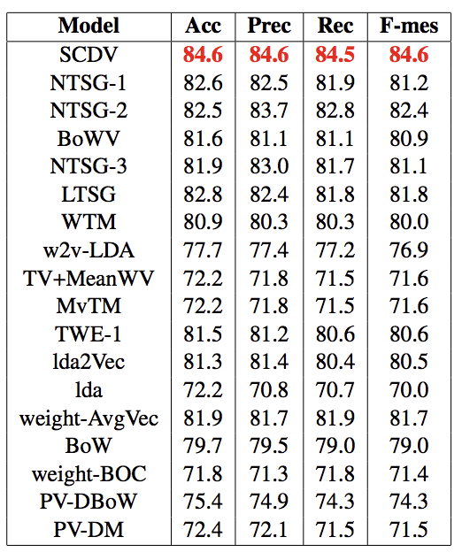
各ベクトル表現手法についてですが、まずNTSGはNeural-Tensor-Skip-Gramという(https://www.ijcai.org/Proceedings/15/Papers/185.pdf) 現状のState-of-the-Artとされていた手法のことです。

skip-gramは単語の組み合わせから文脈を予測することでベクトル表現を獲得し、TWE(Topical Word Embedding)という手法ではそれに加えてトピックも考慮してみようと言う手法です。(https://github.com/largelymfs/topical_word_embeddings これは2015のAAAI)これに対してNTSGでは更にそれら行列をtensor Factorizationで整えてあげるという感じで修正したものです。(あまり自信がない)
その下に来ているBowVというのはBag of Words Vectorsの略で、本論文共著者の中にも入っているVivek氏がやっていたSCDVの前身となる手法です。こちらも根幹は同じですが、ソフトクラスタリングではなくハードクラスタリングで、且つIDF値も考えない手法でした。またスパース化も施さないため、実際にテキスト分類する際のトレーニング時間を考えるとそれなりの時間がかかってしまう、という改善ポイントがあったようです。
取り敢えずトップに近い手法だけ見ましたが、とにかくSCDVはそういうこれまで提案されてきた手法をなぎ倒しているわけです。fasttextとかgloveとか、doc2vecとかと比較していないのは何でなの?という気持ちはありますが...
さて、SCDVの利点としてもう一つ上げられるポイントとして、手軽な計算時間でこれだけの精度を得られるというのがあります。
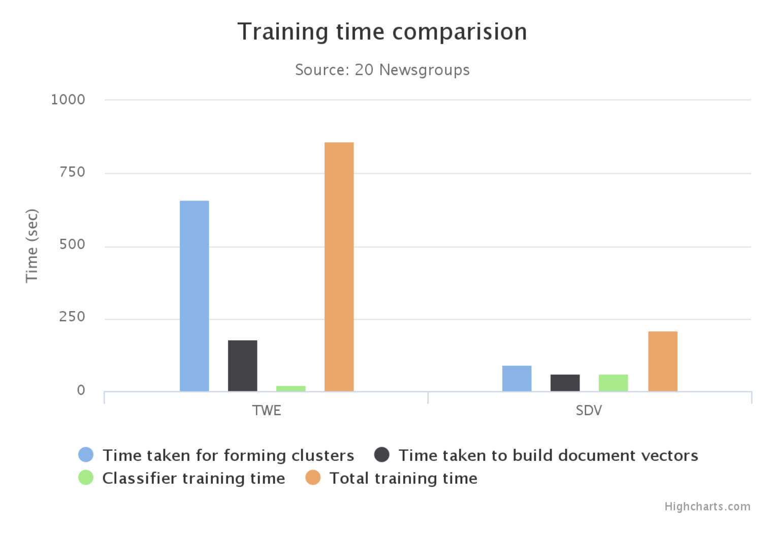
既存手法であるTWEと比較すると計算時間は約三分の一!!!
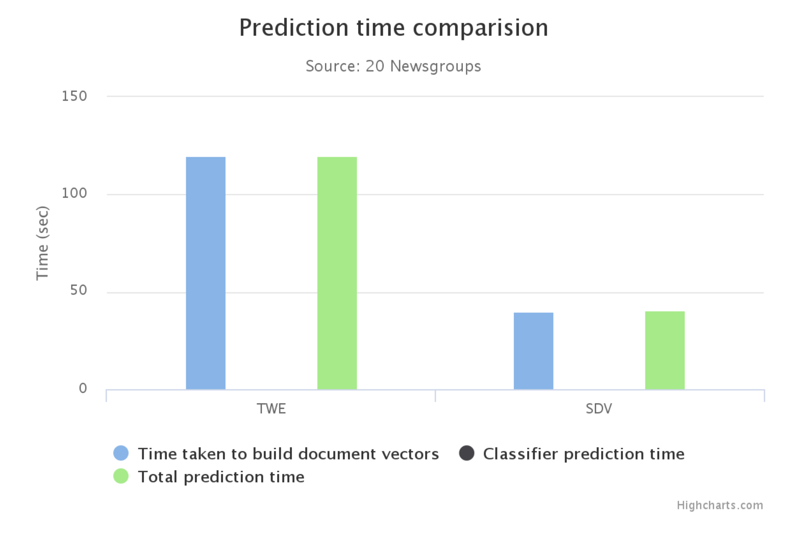
恐らくSVCなのですが、学習から予測に関わる時間はTWEと比較して半分以下!!!
中身のアルゴリズムでやっていること自体はわかりやすいですから時間としてこれだけ既存手法と差が出る、という部分だけ見たら納得ですが、同時に既存手法を上回る精度を出しているというのがすごいところだなと思います。真に強い手法はいつでもシンプルなアーキテクチャから生まれるなあとつくづく思いますね。
日本語コーパスで実験:livedoorニュースコーパスについて
さて、SCDV本体の話はこんなところとして、日本語のコーパスでやって見てどうなるのかを検証してみました。
今回用いたのは冒頭にも示したようにlivedoorニュースコーパスです。中身は9個のニュースサイトから約1000件の記事を引っ張ってきたものになっております。
SCDVがベンチマークの一つとしていた20newsgroupという英語コーパスと構成が似ているので、検証という目的ではばっちりかと。そのうち日本語wikipediaくらいの大規模なコーパスでもやって見なくてはという感じがありますね...
9個のニュースサイトの内訳は次の通り。だいたい名称から内容はわかると思います。わかりづらいのはPeachyとSmaxとかでしょうか。前者はふわふわ女子系の記事、後者はアプリゲームなどの記事を扱っていたメディアです。
| クラス |
|---|
| 独女通信 |
| ITライフハック |
| 家電チャンネル |
| livedoor home |
| movie-enter |
| Peachy |
| Smax |
| スポーツウォッチ |
| トピックニュース |
SCDVのコードはGithubで公開されている(https://github.com/dheeraj7596/SCDV )ほか、ベンチマークとなるデータセットに対する適用方法がそのままあるので、今回のデータセットを使うにあたっては資産をほとんどそのまま使うことができました。python2だった部分をpython3に対応させるのがちょっと手間でしたが...
リポジトリ全体はこちら:
python3に対応させて20newsgroupを実行しているのが
livedoorニュースコーパスで実験しているのが
ノートブック、雑にやってしまったので適宜必要なところはコードを貼っていきながら解説します。
まずはword2vecを学習させる+単語ベクトル空間を可視化
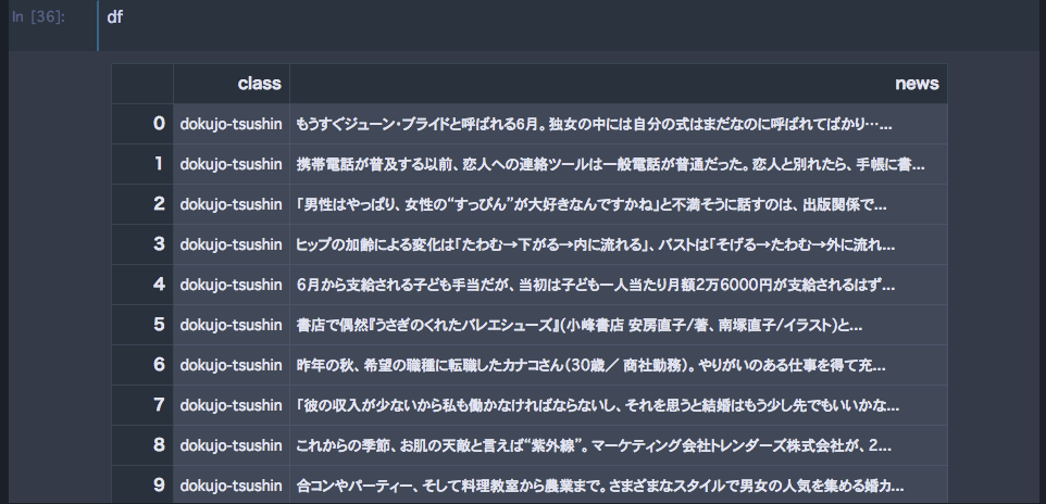
まずはword2vecを学習させていきます。livedoorニュースコーパスはテキストファイルで散らばっているのでそれを一つのデータフレームにするところからです。
import pandas as pd
import glob
import os
from tqdm import tqdm_notebook as tqdm
#preprocessing
dirlist = ["dokujo-tsushin","it-life-hack","kaden-channel","livedoor-homme",
"movie-enter","peachy","smax","sports-watch","topic-news"]
df = pd.DataFrame(columns=["class","news"])
for i in tqdm(dirlist):
path = "../japanese-dataset/livedoor-news-corpus/"+i+"/*.txt"
files = glob.glob(path)
files.pop()
for j in tqdm(files):
f = open(j)
data = f.read()
f.close()
t = pd.Series([i,"".join(data.split("\n")[3:])],index = df.columns)
df = df.append(t,ignore_index=True)
出来上がるデータフレームはこんな感じです。
## create word2vec
import logging
import numpy as np
from gensim.models import Word2Vec
import MeCab
import time
from sklearn.preprocessing import normalize
import sys
import re
start = time.time()
tokenizer = MeCab.Tagger("-Owakati")
sentences = []
print ("Parsing sentences from training set...")
# Loop over each news article.
for review in tqdm(df["news"]):
try:
# Split a review into parsed sentences.
result = tokenizer.parse(review).replace("\u3000","").replace("\n","")
result = re.sub(r'[01234567890123456789!@#$%^&\-|\\*\“()_■×※⇒—●(:〜+=)/*&^%$#@!~`){}…\[\]\"\'\”:;<>?<>?、。・,./『』【】「」→←○]+', "", result)
h = result.split(" ")
h = list(filter(("").__ne__, h))
sentences.append(h)
except:
continue
logging.basicConfig(format='%(asctime)s : %(levelname)s : %(message)s',\
level=logging.INFO)
num_features = 200 # Word vector dimensionality
min_word_count = 20 # Minimum word count
num_workers = 40 # Number of threads to run in parallel
context = 10 # Context window size
downsampling = 1e-3 # Downsample setting for frequent words
print ("Training Word2Vec model...")
# Train Word2Vec model.
model = Word2Vec(sentences, workers=num_workers, hs = 0, sg = 1, negative = 10, iter = 25,\
size=num_features, min_count = min_word_count, \
window = context, sample = downsampling, seed=1)
model_name = str(num_features) + "features_" + str(min_word_count) + "minwords_" + str(context) + "context_len2alldata"
model.init_sims(replace=True)
# Save Word2Vec model.
print ("Saving Word2Vec model...")
model.save("../japanese-dataset/livedoor-news-corpus/model/"+model_name)
endmodeltime = time.time()
print ("time : ", endmodeltime-start)
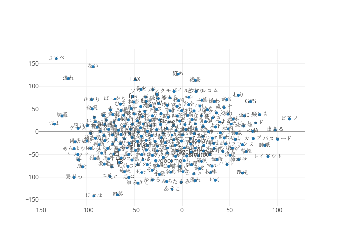
これでword2vecの学習完了です。出来上がったword2vecに対して可視化をやってみます。tSNEで二次元に圧縮。
# plain word2vec t-SNE Visualization
word2vec_model=model
skip=0
limit=241
vocab = word2vec_model.wv.vocab
emb_tuple = tuple([word2vec_model[v] for v in vocab])
X = np.vstack(emb_tuple)
tsne_model = TSNE(n_components=2, random_state=0,verbose=2)
np.set_printoptions(suppress=True)
tsne_model.fit_transform(X)
plain_tsne = pd.DataFrame(tsne_model.embedding_[skip:limit, 0],columns = ["x"])
plain_tsne["y"] = pd.DataFrame(tsne_model.embedding_[skip:limit, 1])
plain_tsne["word"] = list(vocab)[skip:limit]
# plain_tsne["cluster"] = idx[skip:limit] # クラスタを計算し終わったあとならここでクラスタを付与できます
# plain_tsne.plot.scatter(x="x",y="y",c="cluster",cmap="viridis",figsize=(8, 6),s=30)
plain_tsne.plot.scatter(x="x",y="y",figsize=(8, 6),s=30)

https://plot.ly/~fufufukakaka/16/#plot
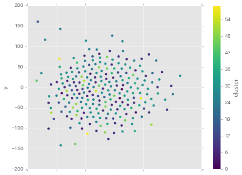
各単語のクラスタで色分けすると次のようになりました。

tsneをかける前にクラスタリングして、そのあと可視化するといつもこんな感じになる気がしますね...
あまりいい感じに分かれているとは言えないですし、いつものことですが単語ごとに孤立していたりそうでなかったりしています。
確率重み付け単語ベクトルを求める+単語ベクトル空間を可視化
ではプレーンなword2vecを元にしてSCDVを求めていきます。
## create gwbowv
from sklearn.feature_extraction.text import TfidfVectorizer,HashingVectorizer
import pickle
from sklearn.mixture import GaussianMixture
from sklearn.preprocessing import LabelEncoder
from sklearn.model_selection import train_test_split
def drange(start, stop, step):
r = start
while r < stop:
yield r
r += step
def cluster_GMM(num_clusters, word_vectors):
# Initalize a GMM object and use it for clustering.
clf = GaussianMixture(n_components=num_clusters,
covariance_type="tied", init_params='kmeans', max_iter=50)
# Get cluster assignments.
clf.fit(word_vectors)
idx = clf.predict(word_vectors)
print ("Clustering Done...", time.time()-start, "seconds")
# Get probabilities of cluster assignments.
idx_proba = clf.predict_proba(word_vectors)
# Dump cluster assignments and probability of cluster assignments.
pickle.dump(idx, open('../japanese-dataset/livedoor-news-corpus/model/gmm_latestclusmodel_len2alldata.pkl',"wb"))
print ("Cluster Assignments Saved...")
pickle.dump(idx_proba,open( '../japanese-dataset/livedoor-news-corpus/model/gmm_prob_latestclusmodel_len2alldata.pkl',"wb"))
print ("Probabilities of Cluster Assignments Saved...")
return (idx, idx_proba)
def read_GMM(idx_name, idx_proba_name):
# Loads cluster assignments and probability of cluster assignments.
idx = pickle.load(open('../japanese-dataset/livedoor-news-corpus/model/gmm_latestclusmodel_len2alldata.pkl',"rb"))
idx_proba = pickle.load(open( '../japanese-dataset/livedoor-news-corpus/model/gmm_prob_latestclusmodel_len2alldata.pkl',"rb"))
print ("Cluster Model Loaded...")
return (idx, idx_proba)
def get_probability_word_vectors(featurenames, word_centroid_map, num_clusters, word_idf_dict):
# This function computes probability word-cluster vectors
prob_wordvecs = {}
for word in word_centroid_map:
prob_wordvecs[word] = np.zeros( num_clusters * num_features, dtype="float32" )
for index in range(0, num_clusters):
try:
prob_wordvecs[word][index*num_features:(index+1)*num_features] = model[word] * word_centroid_prob_map[word][index] * word_idf_dict[word]
except:
continue
# prob_wordvecs_idf_len2alldata = {}
# i = 0
# for word in featurenames:
# i += 1
# if word in word_centroid_map:
# prob_wordvecs_idf_len2alldata[word] = {}
# for index in range(0, num_clusters):
# prob_wordvecs_idf_len2alldata[word][index] = model[word] * word_centroid_prob_map[word][index] * word_idf_dict[word]
# for word in prob_wordvecs_idf_len2alldata.keys():
# prob_wordvecs[word] = prob_wordvecs_idf_len2alldata[word][0]
# for index in prob_wordvecs_idf_len2alldata[word].keys():
# if index==0:
# continue
# prob_wordvecs[word] = np.concatenate((prob_wordvecs[word], prob_wordvecs_idf_len2alldata[word][index]))
return prob_wordvecs
def create_cluster_vector_and_gwbowv(prob_wordvecs, wordlist, word_centroid_map, word_centroid_prob_map, dimension, word_idf_dict, featurenames, num_centroids, train=False):
# This function computes SDV feature vectors.
bag_of_centroids = np.zeros( num_centroids * dimension, dtype="float32" )
global min_no
global max_no
for word in wordlist:
try:
temp = word_centroid_map[word]
except:
continue
bag_of_centroids += prob_wordvecs[word]
norm = np.sqrt(np.einsum('...i,...i', bag_of_centroids, bag_of_centroids))
if(norm!=0):
bag_of_centroids /= norm
# To make feature vector sparse, make note of minimum and maximum values.
if train:
min_no += min(bag_of_centroids)
max_no += max(bag_of_centroids)
return bag_of_centroids
便利な関数群を定義。
num_features = 200 # Word vector dimensionality
min_word_count = 20 # Minimum word count
num_workers = 40 # Number of threads to run in parallel
context = 10 # Context window size
downsampling = 1e-3 # Downsample setting for frequent words
model_name = str(num_features) + "features_" + str(min_word_count) + "minwords_" + str(context) + "context_len2alldata"
# Load the trained Word2Vec model.
model = Word2Vec.load("../japanese-dataset/livedoor-news-corpus/model/"+model_name)
# Get wordvectors for all words in vocabulary.
word_vectors = model.wv.syn0
# Load train data.
train,test = train_test_split(df,test_size=0.3,random_state=40)
all = df
# Set number of clusters.
num_clusters = 60
idx, idx_proba = cluster_GMM(num_clusters, word_vectors)
# Create a Word / Index dictionary, mapping each vocabulary word to
# a cluster number
word_centroid_map = dict(zip( model.wv.index2word, idx ))
# Create a Word / Probability of cluster assignment dictionary, mapping each vocabulary word to
# list of probabilities of cluster assignments.
word_centroid_prob_map = dict(zip( model.wv.index2word, idx_proba ))
ここまでで、各単語空間に対するクラスタリングが完了します。word_centroid_mapは各単語のクラスタを示すdict、word_centroid_prob_mapは各単語のソフトクラスタリングによる各クラスタに属する確率を示すdictになっています。
# Computing tf-idf values.
traindata = []
for review in all["news"]:
result = tokenizer.parse(review).replace("\u3000","").replace("\n","")
result = re.sub(r'[01234567890123456789!@#$%^&\-|\\*\“()_■×※⇒—●(:〜+=)/*&^%$#@!~`){}…\[\]\"\'\”:;<>?<>?、。・,./『』【】「」→←○]+', "", result)
h = result.split(" ")
h = filter(("").__ne__, h)
traindata.append(" ".join(h))
tfv = TfidfVectorizer(dtype=np.float32)
tfidfmatrix_traindata = tfv.fit_transform(traindata)
featurenames = tfv.get_feature_names()
idf = tfv._tfidf.idf_
# Creating a dictionary with word mapped to its idf value
print ("Creating word-idf dictionary for Training set...")
word_idf_dict = {}
for pair in zip(featurenames, idf):
word_idf_dict[pair[0]] = pair[1]
ここではTFIDF値を計算しています。最後にそれをdictにまとめています。
# Pre-computing probability word-cluster vectors.
prob_wordvecs = get_probability_word_vectors(featurenames, word_centroid_map, num_clusters, word_idf_dict)
## 該当する関数を再掲
def get_probability_word_vectors(featurenames, word_centroid_map, num_clusters, word_idf_dict):
# This function computes probability word-cluster vectors
prob_wordvecs = {}
for word in word_centroid_map:
prob_wordvecs[word] = np.zeros( num_clusters * num_features, dtype="float32" )
for index in range(0, num_clusters):
try:
prob_wordvecs[word][index*num_features:(index+1)*num_features] = model[word] * word_centroid_prob_map[word][index] * word_idf_dict[word]
except:
continue
return prob_wordvecs
今まで求めて来た各単語のクラスタ、確率のdictとtfidfのdict、それとword2vecのモデルを用いて確率で重み付けしたword2vecを求めています。やっていることとしては
prob_wordvecs[word][index*num_features:(index+1)*num_features] = model[word] * word_centroid_prob_map[word][index] * word_idf_dict[word]
が理解できさえすればいいんじゃないかなと思います。つまり、各単語ベクトルのその単語のクラスタ、そして各クラスタに属する確率をIDF値と一緒に掛け合わせているわけです。これによってプレーンなword2vecでは200次元だった単語ベクトルはクラスタ数分だけ倍になります。60クラスタだったら12000次元。
論文の趣旨としてはこのあと文書ベクトルを求めるところに行くのですが、その前にこちらでも単語ベクトル空間を可視化してみました。コードはほとんど同じなので省略。
https://plot.ly/~fufufukakaka/18
プレーンなword2vecと比べるとクラスタがめちゃくちゃはっきりしている...!
これは確かに文書ベクトルにも期待が持てそうな感じ。というか、文書ベクトル前提じゃなくてこの確率で重み付けした単語ベクトルだけでもかなり有用そうな感じ。
SCDVを求める
さて最後に文書のベクトルを求める必要がありますので、やっていきます。
# gwbowv is a matrix which contains normalised document vectors.
gwbowv = np.zeros( (train["news"].size, num_clusters*(num_features)), dtype="float32")
counter = 0
min_no = 0
max_no = 0
for review in train["news"]:
# Get the wordlist in each news article.
result = tokenizer.parse(review).replace("\u3000","").replace("\n","")
result = re.sub(r'[01234567890123456789!@#$%^&\-|\\*\“()_■×※⇒—●(:〜+=)/*&^%$#@!~`){}…\[\]\"\'\”:;<>?<>?、。・,./『』【】「」→←○]+', "", result)
h = result.split(" ")
h = filter(("").__ne__, h)
words = h
gwbowv[counter] = create_cluster_vector_and_gwbowv(prob_wordvecs, words, word_centroid_map, word_centroid_prob_map, num_features, word_idf_dict, featurenames, num_clusters, train=True)
counter+=1
if counter % 1000 == 0:
print ("Train News Covered : ",counter)
gwbowv_name = "SDV_" + str(num_clusters) + "cluster_" + str(num_features) + "feature_matrix_gmm_sparse.npy"
gwbowv_test = np.zeros( (test["news"].size, num_clusters*(num_features)), dtype="float32")
counter = 0
for review in test["news"]:
# Get the wordlist in each news article.
result = tokenizer.parse(review).replace("\u3000","").replace("\n","")
result = re.sub(r'[01234567890123456789!@#$%^&\-|\\*\“()_■×※⇒—●(:〜+=)/*&^%$#@!~`){}…\[\]\"\'\”:;<>?<>?、。・,./『』【】「」→←○]+', "", result)
h = result.split(" ")
h = filter(("").__ne__, h)
words = h
gwbowv_test[counter] = create_cluster_vector_and_gwbowv(prob_wordvecs, words, word_centroid_map, word_centroid_prob_map, num_features, word_idf_dict, featurenames, num_clusters)
counter+=1
if counter % 1000 == 0:
print ("Test News Covered : ",counter)
test_gwbowv_name = "TEST_SDV_" + str(num_clusters) + "cluster_" + str(num_features) + "feature_matrix_gmm_sparse.npy"
print ("Making sparse...")
# Set the threshold percentage for making it sparse.
percentage = 0.04
min_no = min_no*1.0/len(train["news"])
max_no = max_no*1.0/len(train["news"])
print ("Average min: ", min_no)
print ("Average max: ", max_no)
thres = (abs(max_no) + abs(min_no))/2
thres = thres*percentage
# Make values of matrices which are less than threshold to zero.
temp = abs(gwbowv) < thres
gwbowv[temp] = 0
temp = abs(gwbowv_test) < thres
gwbowv_test[temp] = 0
#saving gwbowv train and test matrices
np.save("../japanese-dataset/livedoor-news-corpus/model/"+gwbowv_name, gwbowv)
np.save("../japanese-dataset/livedoor-news-corpus/model/"+test_gwbowv_name, gwbowv_test)
文書ベクトルの可視化
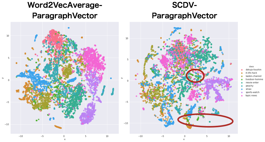
では、SCDVが手に入ったところで、プレーンword2vecでの文書ベクトルと、SCDVでの可視化を比較してみましょう。
プレーンword2vecによる文書ベクトル可視化
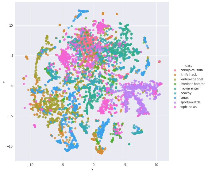
まずはプレーンword2vecの単語ベクトル平均で表した文書ベクトルの可視化結果から。
import seaborn as sns
#document vector visualization
## plain word2vec
def plain_word2vec_document_vector(sentence,word2vec_model,num_features):
bag_of_centroids = np.zeros(num_features, dtype="float32")
for word in sentence:
try:
temp = word2vec_model[word]
except:
continue
bag_of_centroids += temp
bag_of_centroids = bag_of_centroids / len(sentence)
return bag_of_centroids
plainDocVec_all = {}
counter = 0
num_features = 200
for review in all["news"]:
# Get the wordlist in each news article.
result = tokenizer.parse(review).replace("\u3000","").replace("\n","")
result = re.sub(r'[01234567890123456789!@#$%^&\-|\\*\“()_■×※⇒—●(:〜+=)/*&^%$#@!~`){}…\[\]\"\'\”:;<>?<>?、。・,./『』【】「」→←○]+', "", result)
h = result.split(" ")
h = filter(("").__ne__, h)
words = list(h)
plainDocVec_all[counter] = plain_word2vec_document_vector(words,word2vec_model,num_features)
counter+=1
if counter % 1000 == 0:
print ("All News Covered : ",counter)
## visualize all document vector
emb_tuple = tuple([plainDocVec_all[v] for v in plainDocVec_all.keys()])
X = np.vstack(emb_tuple)
plain_w2v_doc= TSNE(n_components=2, random_state=0,verbose=2)
np.set_printoptions(suppress=True)
plain_w2v_doc.fit(X)
alldoc_plainw2v_tsne = pd.DataFrame(plain_w2v_doc.embedding_[:, 0],columns = ["x"])
alldoc_plainw2v_tsne["y"] = pd.DataFrame(plain_w2v_doc.embedding_[:, 1])
alldoc_plainw2v_tsne["class"] = list(all["class"])
sns.lmplot(data=alldoc_plainw2v_tsne,x="x",y="y",hue="class",fit_reg=False,size=8)

素直にseaborn使う方がやっぱり散布図での色分けがしやすいなふと思い、ここではseabornで描画しています。
クラスタと合わせてみると、そこまで悪そうな結果ではないっぽいですね。概ねまとまっていると思いますが、ちょいちょい飛び地的な文書ベクトルがあるようです。
SCDVによる文書ベクトル可視化
ではSCDVの結果も見てみましょう。
あれ?なんかプレーンなword2vecで作った文書ベクトルの方がうまくわかれていたような... むしろこれだと一緒くたになっているように見えますが大丈夫でしょうか...
と一瞬思ったのですが、よくよくカテゴリごとの特性を考えてみると
- 一番散らばっているピンクはトピックニュース...分野を限定しないブレイキングニュースなどが主なので、色々なカテゴリに広がるのは間違っていないというかむしろそうあるべき
- 青色のsmaxと橙のITライフハック、黄緑の家電チャンネルは混ざり合っている...内容を考えれば混ざっていても不自然ではない
- 赤色の独女通信、紫色のスポーツウォッチはそんなに散らばっていない...せやなという感じ
- 青緑のpeachyが独女通信に近い位置に移動...より納得できる位置になった
- 緑色のlivedoor-homeも分散...内容的には世間話みたいな感じなのでトピックニュースと近い?
- movie-enterも独女通信に近いところに移動?...色的に差分が分かりづらいですが、おそらく移動しています。これはちょっとわからなかった。
ちなみにlivedoor-homeの一文目はこんな感じです(なぜか落として来た時点でlivedoor-hommeという謎のラベルだった)。そんなにトピックにまとまりはなさそうですよね。
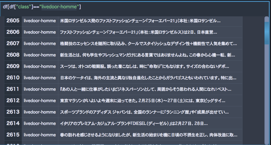
20newsgroup datasetはニュースのカテゴリ、ということではっきり分かれていることを前提におけるデータセットだと思うのですが、それに対してこちらのコーパスは異なるメディアからの記事取得ということなのでこういう分布になってしまうのでしょう。
そう考えるとじゃあちゃんとトピック的に分かれたデータセットじゃないとSCDVって効果が出ないのでは、という気持ちも出て来ます...うーん、どうなんでしょうか。まあ検証してみましょう。
テキスト分類の精度
元論文ではSVCでしたが時間がかかってしょうがないので、LightGBMでやりました。時間もかけたくなかったので、何も設定していない素のLGBMClassifierでやっています。多クラス分類なので、目的パラメータだけ整えておきました。
## test lgb
from sklearn.metrics import classification_report
import lightgbm as lgb
start = time.time()
clf = lgb.LGBMClassifier(objective="multiclass")
clf.fit(gwbowv, train["class"])
Y_true, Y_pred = test["class"], clf.predict(gwbowv_test)
print ("Report")
print (classification_report(Y_true, Y_pred, digits=6))
print ("Accuracy: ",clf.score(gwbowv_test,test["class"]))
print ("Time taken:", time.time() - start, "\n")
これに対して、プレーンなword2vecの平均、fasttextでも単語のベクトルを平均したものを文書ベクトルとして、また、doc2vecでも文書ベクトルを取得し、同じコードで精度を求めてみました。比較した表がこちら。全てlightgbmでの結果です。なお、SCDVの元コードの時点でtrain,testが分けられていたため、こちらも同様にホールドアウト検証法での精度となります。CVじゃなくてごめんなさい。
| method | accuracy | precision | recall | f1 |
|---|---|---|---|---|
| SCDV | 0.8742 | 0.8743 | 0.8742 | 0.8730 |
| fastext-average | 0.8588 | 0.8580 | 0.8588 | 0.8576 |
| doc2vec | 0.8398 | 0.8386 | 0.8398 | 0.8385 |
| word2vec-average | 0.8249 | 0.8221 | 0.8249 | 0.8217 |
え、いやまじですか?正直ここまで差がつくとは思っていませんでした。word2vecの単語ベクトル平均と比較すると実に5%も差がつくという。これはなかなか大きい結果ではないでしょうか。
そういえば、doc2vecはparagraoh vectorを意識した手法のはずなのに、fasttextの単語ベクトル平均に負けてしまっています。かわいそう。
sklearn.metrics.classification_reportで各クラスごとの成績も見てみます。ここではword2vec-averageとSCDVを比較します。
SCDVの各クラス分類精度
| class | precision | recall | f1-score | support |
|---|---|---|---|---|
| dokujo-tsushin | 0.7947 | 0.8486 | 0.8208 | 251 |
| it-life-hack | 0.8360 | 0.8427 | 0.8393 | 248 |
| kaden-channel | 0.8875 | 0.8554 | 0.8711 | 249 |
| livedoor-home | 0.8545 | 0.6438 | 0.7343 | 146 |
| movie-enter | 0.9179 | 0.9389 | 0.9283 | 262 |
| peachy | 0.7992 | 0.7992 | 0.7992 | 254 |
| smax | 0.9632 | 0.9886 | 0.9757 | 265 |
| sports-watch | 0.8770 | 0.9428 | 0.9087 | 280 |
| topic-news | 0.9233 | 0.8945 | 0.9087 | 256 |
| avg / total | 0.8743 | 0.8742 | 0.8730 | 2211 |
word2vec-averageの各クラス分類精度
| class | precision | recall | f1-score | support |
|---|---|---|---|---|
| dokujo-tsushin | 0.8023 | 0.8247 | 0.8133 | 251 |
| it-life-hack | 0.8208 | 0.7943 | 0.8073 | 248 |
| kaden-channel | 0.8127 | 0.7670 | 0.7892 | 249 |
| livedoor-home | 0.72 | 0.4931 | 0.5853 | 146 |
| movie-enter | 0.8530 | 0.9083 | 0.8798 | 262 |
| peachy | 0.7568 | 0.7598 | 0.7583 | 254 |
| smax | 0.9202 | 0.9584 | 0.9390 | 265 |
| sports-watch | 0.8630 | 0.9 | 0.8811 | 280 |
| topic-news | 0.7971 | 0.8593 | 0.8270 | 256 |
| avg / total | 0.8221 | 0.8249 | 0.8217 | 2211 |
考察
こうしてみると、f1では完全に圧勝ですね。特に、livedoor-homeの上がり方が凄まじい。先ほど可視化したプレーンword2vecによる文書ベクトル空間を見てみると、確かにlivedoor-homeは一箇所に固まってはいましたが他のクラスタとの距離が近く埋没し気味にも見えます。それがSCDVになると、いくらか見えるようになっていると解釈できそうな気がします。
逆に上がり幅が少なかったクラスとしては独女通信やスポーツウォッチが2%程度の上昇にとどまっています。おそらくこれは、プレーンword2vecで構築した文書ベクトルの時点で既にクラスタがはっきりしていたので、SCDVによる恩恵を受けにくかったのではないかと推察できます。精度が上がったのは近かったクラスタとの差がいくらかはっきりしたことによるものではないでしょうか。
まとめと感じた課題など
というわけで、非常に単純なアイデアでお手軽に高い精度を得られるSCDVは日本語コーパスでも同様に精度向上を見込めることがわかりました。
今回試したコーパスは前述したようにはっきりと内容が分かれているとは言い難い部分もあったにもかかわらず、精度向上を確認することができたのでとても満足です。次はwikipediaコーパスの主要カテゴリ(科学、学問、歴史など)の9クラスでもやってみたいですね。
また、SCDVを構成する確率で重み付けした単語ベクトル自体も非常に有用そうでした。今回はコサイン類似度である単語に対してどのような単語が返ってくるように変化するのかの検証はできませんでしたが、tSNEで可視化した結果を見る限りとても期待が持てそうです。wikipediaで学習したそのベクトルを、LSTMなどディープ系の手法のembedding層に埋め込むことで精度向上が望めるんじゃないかなと。
SCDVを改善するとしたら何ができるんでしょうね... 既存手法のTWEはトピックを考慮するぞということでLDAを併用したメソッドでしたが、SCDVはTFIDFで恐らくトピックベクトルを与えている、という解釈です。であれば、TFIDFではなくLDAではどうなるんだろう?という疑問も出てくるわけですね。
また今回検証の結果でfasttext-averageとの差がそんなになかったということもを踏まえると、word2vecではなくfasttextをベースにSCDVを構築する方が良いと思われます、日本語でこれだったわけですから、英語ならさらに精度が上がるんじゃないでしょうか。
wikipediaで学習させる、fasttext版のSCDVを試す、両者をpythonのコードにまとめてgensimのword2vecみたいなメソッドを用意して使えるようにする、などが今後のTodoっぽいかなあ。やっていきます
