はじめに
2時限目は機械学習のプログラミングを強力にサポートしてくれるライブラリの使い方を学んでいきます。
1. NumPyを使った線形代数の演算
まずはNumPyというライブラリを使って、線形代数のプログラミングに慣れましょう。
NumPyとは?
- 行列計算や大規模な多次元配列を取り扱うためのPythonの拡張モジュール
- NumPyの内部はC言語で書かれているため、通常のPythonより高速に動作する
基本的な使い方
numpyモジュールをインポートして使います。
import numpy as np # npと略されることが多いです

a = np.array([1, 2])
print(a) # => [1 2]
線形代数の演算
以下のような線形代数の演算をプログラミングしていきます。
- ベクトル・行列
- ベクトル・行列の演算
- 転置
- 単位行列
- 逆行列
ベクトル・行列
a = np.array([[1, 2, 3]]) # 長さ3の横ベクトル
B = np.array([[1, 2], [3, 4]]) # 2*2の行列
C = np.array(((4, 5, 6), np.array([7, 8, 9]))) # タプルやnp.ndarrayでも生成可能

# np.ndarrayのよく使う属性
print(C.ndim) # => 2 次元数
print(C.size) # => 6 全体の要素数
print(C.shape) # => (2, 3) 各次元の要素数
print(C.dtype) # => int64 各要素のデータ型
その他にも、以下のようなベクトル・行列の生成方法があります。
a = np.zeros([1, 2]) # 要素が0の横ベクトル
B = np.ones([2, 3]) # 要素が1の行列
C = np.identity(3) # 単位行列
ベクトル・行列内の要素へのアクセスは以下のようになります。
A = np.array(((4, 5, 6), np.array([7, 8, 9])))
A[0] # => [4 5 6]
A[1][1:2] # => [8]
問題1
- 以下の縦ベクトルを生成するプログラムを書いてください。
\boldsymbol{x} =
\begin{bmatrix}
1 \\
2 \\
3
\end{bmatrix}
問題1の答え
x = np.array([[1], [2], [3]])
ベクトル・行列の演算
A = np.array([[1, 2], [3, 4]]) # 行列を生成
B = np.array([[5, 6], [7, 8]])

A + B # 加算
A - B # 減算
A * B # 要素同士の積
np.dot(A, B) # 行列積
問題2
- 以下の計算をしてください。
(1)
\begin{bmatrix}
1 &
2 &
3
\end{bmatrix}
\begin{bmatrix}
1 \\
2 \\
3
\end{bmatrix}
(2)
\begin{bmatrix}
1 & 2 \\
2 & 3
\end{bmatrix}
\begin{bmatrix}
4 & 5 & 6 \\
2 & 7 & 3
\end{bmatrix}
問題2の答え
# (1)
x1 = np.array([[1, 2, 3]])
x2 = np.array([[1], [2], [3]])
np.dot(x1, x2) # => array([[14]])

# (2)
A = np.array([[1, 2], [2, 3]])
B = np.array([[4, 5, 6], [2, 7, 3]])
np.dot(A, B) # => array([[ 8, 19, 12],
             #           [14, 31, 21]])
### 転置行列・転置ベクトル

```python
A = np.array([[1, 2], [3, 4]])
b = np.array([[1, 2, 3]])

print(A.T)
# => [[1 3]
#     [2 4]]

print(b.T)
# => [[1]
#     [2]
#     [3]]
問題3
- 行列$A,B$が以下のとき、$(1)$の等式を満たすか確認してください。
A=
\begin{bmatrix}
1 & 2 \\
3 & 4
\end{bmatrix}
, B=
\begin{bmatrix}
5 & 6 \\
7 & 8
\end{bmatrix}
(AB)^{T} = B^{T} A^{T}
問題3の答え
A = np.array([[1, 2], [3, 4]])
B = np.array([[5, 6], [7, 8]])

print(np.dot(A, B).T)
print(np.dot(B.T, A.T))
実行結果
>>> print(np.dot(A, B).T)
[[19 43]
 [22 50]]
>>> print(np.dot(B.T, A.T))
[[19 43]
 [22 50]]
ランク(階数)
numpy.linalgパッケージを利用して次のように計算します。
A = np.array([[1, 2], [3, 4]])
print(np.linalg.matrix_rank(A)) # => 2
逆行列
逆行列もnumpy.linalgパッケージを利用します。
A = np.array([[1, 2], [3, 4]])
AINV = np.linalg.inv(A)
print(AINV)
# => [[-2.   1. ]
#     [ 1.5 -0.5]]
問題4
- 上記の行列に関して、以下を計算して単位行列になるか確認してください。
A A^{-1}
問題4の答え
A = np.array([[1, 2], [3, 4]])
AINV = np.linalg.inv(A)

np.dot(A, AINV)
行列式
行列式も同様にnumpy.linalgパッケージを利用して求めることができます。
A = np.array([[1, 2], [3, 4]])
print(np.linalg.det(A))
# => -2.0
2. pandasを使ったデータ操作
次に、pandasというライブラリを使って、機械学習で用いるデータの操作方法について学びます。
pandasとは?
- Pythonでデータ分析・操作を行うのによく使われるライブラリ
-
SeriesとDataFrameの2種類のデータ構造があります -
Seriesは1次元のデータを、DataFrameはSeriesが集まった2次元の表のようなものと考えてください
基本的な使い方
import pandas as pd # pdと略すことが多いです
s = pd.Series([1, 2, 3, 4, 5, 6])
print(s)
# => 0    1
#    1    2
#    2    3
#    3    4
#    4    5
#    5    6
#    dtype: int64

df = pd.DataFrame(
    {'name': ['一郎', '隆', '健介', '花子', '亜紀', '恵'],
     'age': [29, 24, 22, 18, 20, 23],
     'sex': ['m', 'm', 'm', 'f', 'f', 'f']})
print(df)
# =>    age name sex
#    0   29   一郎   m
#    1   24    隆   m
#    2   22   健介   m
#    3   18   花子   f
#    4   20   亜紀   f
#    5   23    恵   f
pandasを使ってやること
pandasには様々な機能がありますが、今回は以下のステップに絞って学習していきます。
- CSVの読み込み
- ラベリング
- 説明変数(入力変数)の抽出
- 目的変数(出力変数)の抽出
3, 4で抽出した変数を、NumPyや、後の講義で登場するscikit-learnなどの機械学習ライブラリに渡してモデルの学習を行うという流れです。
1. CSVの読み込み
CSVファイルからデータを読み込みます。
df = pd.read_csv('https://archive.ics.uci.edu/ml/machine-learning-databases/iris/iris.data', header=None)
df.tail(3) # データの末尾3列を表示(デフォルトは5)
問題1
- 上記コマンドを実行してください。
-
df.head(n)(nは1以上の整数)を実行してください。
問題1の答え
省略
2. ラベリング
各列にラベルを付与します。
df.columns = ['sepal width', 'sepal length', 'petal width', 'petal length', 'class']
df['sepal width'].head(3) # ラベル名で各列を取得できるようになります
| 0 | 5.1 |
| 1 | 4,9 |
| 2 | 4.7 |
問題2
- 上記を実行してください。
問題2の答え
省略
3. 説明変数(入力変数)の抽出
データから説明変数を抽出します。
X = df[['sepal width', 'sepal length', 'petal width', 'petal length']].values
print(X[0:5])
# => [[ 5.1  3.5  1.4  0.2]
#     [ 4.9  3.   1.4  0.2]
#     [ 4.7  3.2  1.3  0.2]
#     [ 4.6  3.1  1.5  0.2]
#     [ 5.   3.6  1.4  0.2]]
問題3
- 上記を実行してください。
問題3の答え
省略
4. 目的変数(出力変数)の抽出
最後に、データから目的変数を抽出します。
y = df['class'].values
print(y[0:5])
# => ['Iris-setosa' 'Iris-setosa' 'Iris-setosa' 'Iris-setosa' 'Iris-setosa']
問題4
- 上記を実行してください。
- https://archive.ics.uci.edu/ml/machine-learning-databases/housing/ をデータとして、これまでの手順を復習してください。説明変数、目的変数として使うデータは適当でかまいません。
問題4の答え
省略
3. matplotlibを使った可視化
最後はmatplotlibを使って、色々なグラフを描画する方法を学んでいきます。
matplotlibとは?
- Pythonでグラフを描画するときによく使われるライブラリ
-
pyplotモジュールというインターフェースを通じて使われることが多い
%matplotlib inline
import numpy as np
import matplotlib.pyplot as plt # pltと略すことが多いです
N = 100
x = np.random.rand(N)
y = np.random.rand(N)
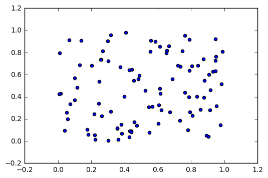
plt.scatter(x, y) # 散布図をプロット
plt.show()
※ %matplotlib inlineはJupyter Notebookでグラフを表示するのに必要
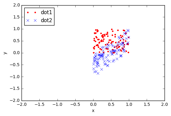
散布図
N = 100
x = np.random.rand(N)
y = np.random.rand(N)
y2 = x + np.random.rand(N) - 1
plt.plot(x, y, c='r', marker='.', linestyle='', label='dot1') # グラフのプロット
plt.plot(x, y2, c='b', marker='x', linestyle='', label='dot2') # グラフのプロット
plt.xlabel('x') # x軸のラベル
plt.ylabel('y') # y軸のラベル
plt.xlim(-2., 2.) # x軸の上限・下限
plt.ylim(-2., 2.) # y軸の上限・下限
plt.legend(loc='upper left') # 凡例の表示
plt.show()
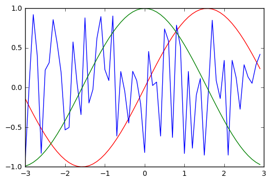
折れ線グラフ
N = 100

x = np.arange(-3, 3, .1) # 0.1刻みで[-3., 3.]のリストを生成
y = np.sin(x) # sin関数
y2 = np.random.rand(N) * 2 - 1
y3 = np.cos(x) # cos関数
plt.plot(x, y, c='r')
plt.plot(x, y2[:60], c='b') # xとyは要素数を揃える必要がある
plt.plot(x, y3, c='g')
plt.show()
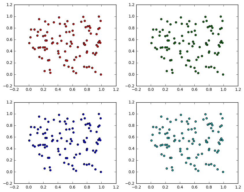
複数の図のプロット
N = 100

x = np.random.rand(N)
y = np.random.rand(N)

plt.figure(figsize=(10, 8))
plt.subplot('221') # 2行2列に分割したうちの1つ目
plt.scatter(x, y, c='r')
plt.subplot('222')
plt.scatter(x, y, c='g')
plt.subplot('223')
plt.scatter(x, y, c='b')
plt.subplot('224')
plt.scatter(x, y, c='c')
plt.show()
その他
- matplotlibのギャラリーを参照 http://matplotlib.org/gallery.html