深層学習 を 用いた 異常値検知 手法まとめ 〜 (Denosing) AutoEncoder, LSTM, TDA（Topological Data Analysis) + CNN

オーソドックス な アプローチ（一般的手法）

まず は、以下 が よくまとまっている。

• 株式会社クロスコンパス・インテリジェンス（2016.10.5）「NVIDIA GPU TECHNOLOGY CONFERENCE JAPAN 2016 Industry Deep Learning」

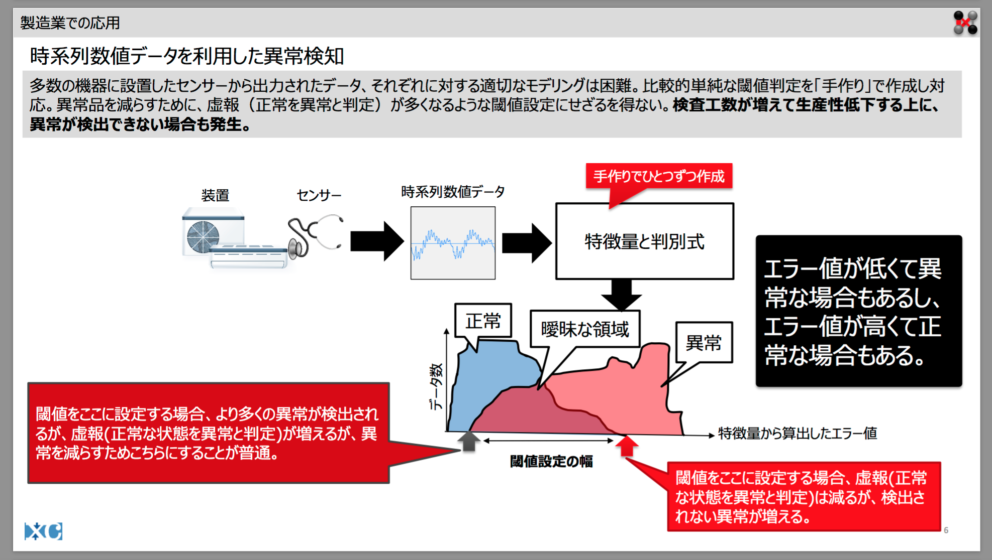
異常値予測 を 行う アプローチ としては、以下 が 一般的な考え方 の ようだ。

• （データ量の多い）正常時のデータ挙動の特徴パターンを学ばせて、
• 新規データが上記の特徴パターンから乖離している場合を、異常とみなす

上記のアプローチをとる理由 は、「異常発生時のデータ」の取得可能件数 は、「正常時のデータ」 に 比べて、取得できるデータの件数 が 圧倒的に少ない から である。

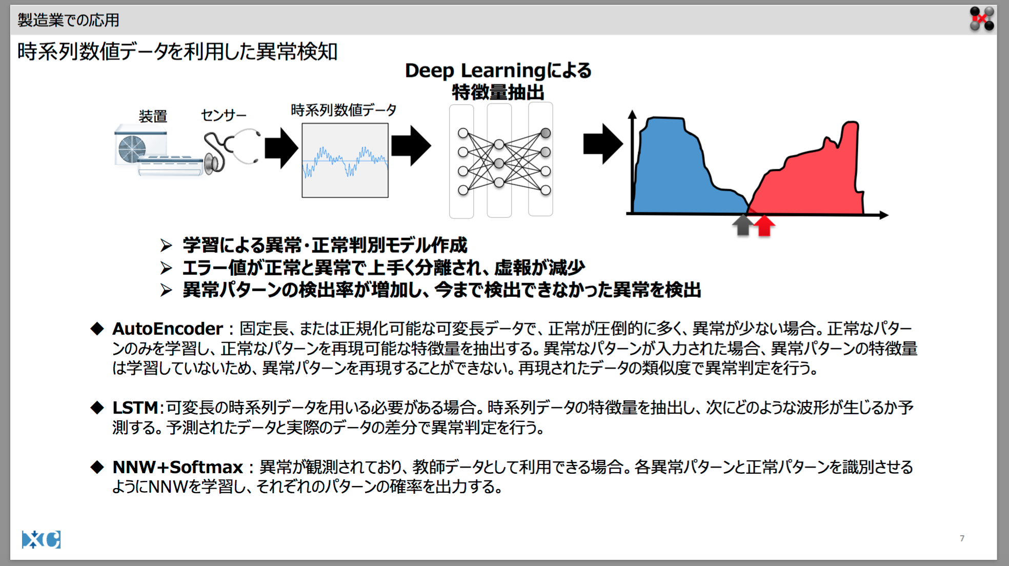
上記のスライド で 挙げられている AutoEncoderモデル や LSTMモデル を 採用し、

• 【 モデル学習段階 】

データ量の多い「正常時の（学習用）データ」のみ を モデル に 与えること

• 【 モデル精度検証（評価）段階 】

• （学習時に与えなかった）「正常期間中のデータ」 及び 「異常期間中のデータ」 を 入力する
• モデル出力値 と 入力した値 との 類似度 （入力値と出力値の類似度） が 低ければ、入力したデータ は、モデル に よって「異常」と判定した もの と みなす。
• モデル出力値 と 入力した値 との 類似度 （入力値と出力値の類似度） が 高ければ、入力したデータ は、モデル に よって「正常」と判定した もの と みなす。

上記 に より、「異常発生時のデータ」の件数の少なさ に起因するモデル学習の困難さ を 回避すること が できる。

「異常」学習 及び 検証用データ の 件数が少ないので、従来の「２値分類モデル」 の採用 は 困難

「異常」（anomaly）とは、たまに発生するものだから、「正常」より 累積発生時間 は少ないの が 通常 で ある。

（そもそも言葉の定義として、発生期間が稀で、特異な状態 が、「異常」と定義される）

従って、学習用 及び 検証用データセット として、「異常発生時」の「正例データ」の取得可能件数は、「正常時のデータ」（負例データ）の取得可能件数 よりも 圧倒的 に 少なくなる。

従って、

モデル学習段階 で、

• 【 正例データ 】「異常発生時」の学習用データ

• 説明変数カラム値（複数）
• 目的変数カラム値（例えば、「異常」＝１）（１カラム）

• 【 負例データ 】「正常状態下」の学習用データ

• 説明変数カラム値（複数）
• 目的変数カラム値（例えば、「正常」＝０）（１カラム）

を 同じデータ件数 学習させて、

モデル検証段階 で、

• 学習時 に モデル に 与えなかった 「異常発生時」の「説明変数」データ（検証用データ） を モデル に 入力

• モデル から 出力される 「目的変数」の推定値（予測値）と、検証用データの実際の目的変数 とが一致する割合 を、

• 「予測」
• 「適合率」
• 「再現率」
• 「F値」
• 「ROC曲線」（ROC Curve）
• 「適合率・再現率曲線」Precision-Recall Curve

として 取りまとめる。

という従来のアプローチ は、学習用 及び 検証用 の「正例データ」 の データ件数の確保の困難さ から、現実的 に 採用することが困難 と なる場合 が 多い。

【 事例① 】AutoEncoder モデル を 用いた 異常値検知モデル

• Anomaly Detection: Increasing Classification Accuracy with H2O's Autoencoder and R

（ 以下、上記ウェブページ より 転載 ）

full source code

# install.packages("h2o")

# point to the prostate data set in the h2o folder - no need to load >h2o in memory yet
prosPath = system.file("extdata", "prostate.csv", package = "h2o")
prostate_df <- read.csv(prosPath)

# We don't need the ID field
prostate_df <- prostate_df[,-1]
summary(prostate_df)

set.seed(1234)
random_splits <- runif(nrow(prostate_df))
train_df <- prostate_df[random_splits < .5,]
dim(train_df)

validate_df <- prostate_df[random_splits >=.5,]
dim(validate_df)

# Get benchmark score

# install.packages('randomForest')
library(randomForest)

outcome_name <- 'CAPSULE'
feature_names <- setdiff(names(prostate_df), outcome_name)
set.seed(1234)
rf_model <- randomForest(x=train_df[,feature_names],
                        y=as.factor(train_df[,outcome_name]),
                        importance=TRUE, ntree=20, mtry = 3)

validate_predictions <- predict(rf_model, >newdata=validate_df[,feature_names], type="prob")


# install.packages('pROC')
library(pROC)
auc_rf = >roc(response=as.numeric(as.factor(validate_df[,outcome_name]))-1,
            predictor=validate_predictions[,2])

plot(auc_rf, print.thres = "best", >main=paste('AUC:',round(auc_rf$auc[[1]],3)))
abline(h=1,col='blue')
abline(h=0,col='green')

# build autoencoder model

library(h2o)
localH2O = h2o.init()
prostate.hex<-as.h2o(train_df, destination_frame="train.hex")
prostate.dl = h2o.deeplearning(x = feature_names, training_frame = >prostate.hex,
                              autoencoder = TRUE,
                              reproducible = T,
                              seed = 1234,
                              hidden = c(6,5,6), epochs = 50)

# interesting per feature error scores
# prostate.anon = h2o.anomaly(prostate.dl, prostate.hex, >per_feature=TRUE)
# head(prostate.anon)

prostate.anon = h2o.anomaly(prostate.dl, prostate.hex, >per_feature=FALSE)
head(prostate.anon)
err <- as.data.frame(prostate.anon)

# interesting reduced features (defaults to last hidden layer)
# >http://www.rdocumentation.org/packages/h2o/functions/h2o.deepfeatures
# reduced_new  <- h2o.deepfeatures(prostate.dl, prostate.hex)

plot(sort(err$Reconstruction.MSE))

# use the easy portion and model with random forest using same >settings

train_df_auto <- train_df[err$Reconstruction.MSE < 0.1,]

set.seed(1234)
rf_model <- randomForest(x=train_df_auto[,feature_names],
                        y=as.factor(train_df_auto[,outcome_name]),
                        importance=TRUE, ntree=20, mtry = 3)

validate_predictions_known <- predict(rf_model, >newdata=validate_df[,feature_names], type="prob")

auc_rf = >roc(response=as.numeric(as.factor(validate_df[,outcome_name]))-1,
            predictor=validate_predictions_known[,2])

plot(auc_rf, print.thres = "best", >main=paste('AUC:',round(auc_rf$auc[[1]],3)))
abline(h=1,col='blue')
abline(h=0,col='green')

# use the hard portion and model with random forest using same >settings
train_df_auto <- train_df[err$Reconstruction.MSE >= 0.1,]

set.seed(1234)
rf_model <- randomForest(x=train_df_auto[,feature_names],
                        y=as.factor(train_df_auto[,outcome_name]),
                        importance=TRUE, ntree=20, mtry = 3)

validate_predictions_unknown <- predict(rf_model, >newdata=validate_df[,feature_names], type="prob")
auc_rf = >roc(response=as.numeric(as.factor(validate_df[,outcome_name]))-1,
            predictor=validate_predictions_unknown[,2])

plot(auc_rf, print.thres = "best", >main=paste('AUC:',round(auc_rf$auc[[1]],3)))
abline(h=1,col='blue')
abline(h=0,col='green')

# bag both results set and measure final AUC score
valid_all <- (validate_predictions_known[,2] + >validate_predictions_unknown[,2]) / 2
auc_rf = >roc(response=as.numeric(as.factor(validate_df[,outcome_name]))-1,
            predictor=valid_all)

plot(auc_rf, print.thres = "best", >main=paste('AUC:',round(auc_rf$auc[[1]],3)))
abline(h=1,col='blue')
abline(h=0,col='green')

• ADVERSARIAL.AI, Deep Learning Approach to Fraud

• Jinwon An and Sungzoon Cho, Variational Autoencoder based Anomaly Detection using Reconstruction Probability

Abstract
We propose an anomaly detection method using the reconstruction probability from the variational auto encoder.

The reconstruction probability is a probabilistic measure that takes into account the variability of the distribution of variables. >
The reconstruction probability has a theoretical background making it a more principled and objective anomaly score than the reconstruction error, which is used by autoencoder and principal components based anomaly detection methods.

Experimental results show that the proposed method outper- forms autoencoder based and principal components based methods.

Utilizing the generative characteristics of the variational autoencoder enables deriving the reconstruction of the data to analyze the underlying cause of the anomaly.

• Olga Lyudchik, Outlier detection using auto encoders

• Shuangfei Zhai, Yu Cheng, Weining Lu and Zhongfei (Mark) Zhang, Deep Structured Energy Based Models for Anomaly Detection

in this work, we propose deep structured energy based models (DSEBMs).

Our approach falls into the category of energy based models (EMBs) (LeCun et al., 2006), which is a powerful tool for density estimation.

An EBM works by coming up with a specific parameterization of the negative log probability, which is called energy, and then computing the density with a proper normalization.

In this work, we focus on deep energy based models (Ngiam et al., 2011), where the energy function is composed of a deep neural network.

Moreover, we investigate various model architectures as to accommodate different data structures.

For ex- ample, for data with static vector inputs, standard feed for- ward neural networks can be applied. However, for sequen- tial data, such as audio sequence, recurrent neural networks (RNNs) are known to be better choices. Likewise, convolutional neural networks (CNNs) are significantly more efficient at modeling spatial structures (Krizhevsky et al., 2012), such as on images. Our model thus allows the en- ergy function to be composed of deep neural networks with designated structures (fully connected, recurrent or convo- lutional), significantly extending the application of EBMs to a wide spectrum of data structures.

• Takaaki Tarawa, Yukihiro TadokoroTOYOTA CENTRAL R&D LABS., INC), Takehisa Yairi(RCAST, University of Tokyo), Structured Denoising Autoencoder for Fault Detection and Analysis

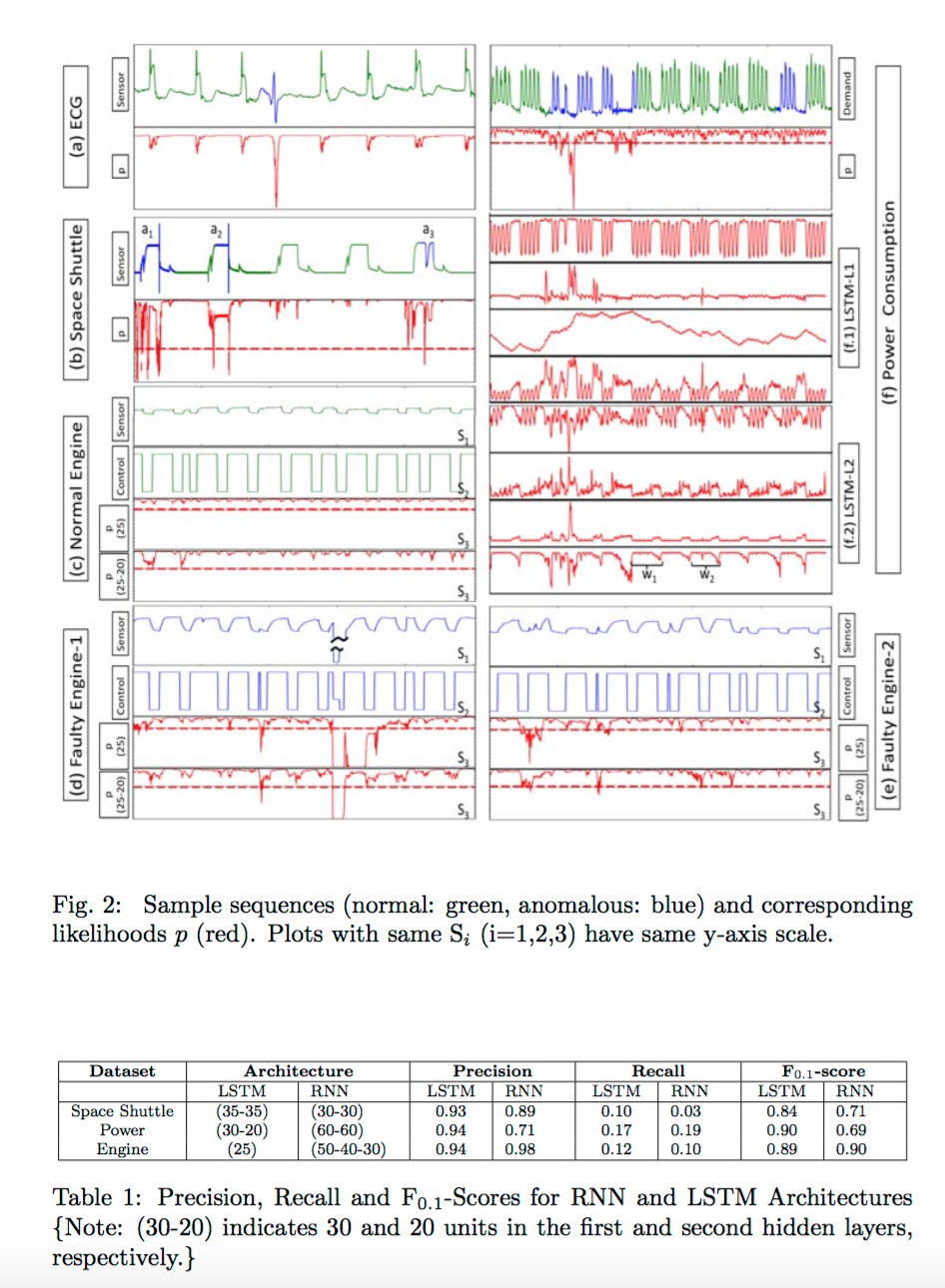
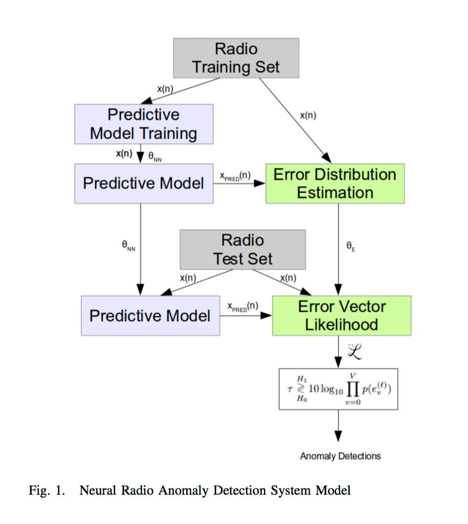
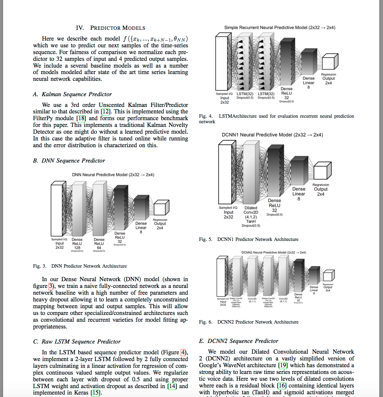
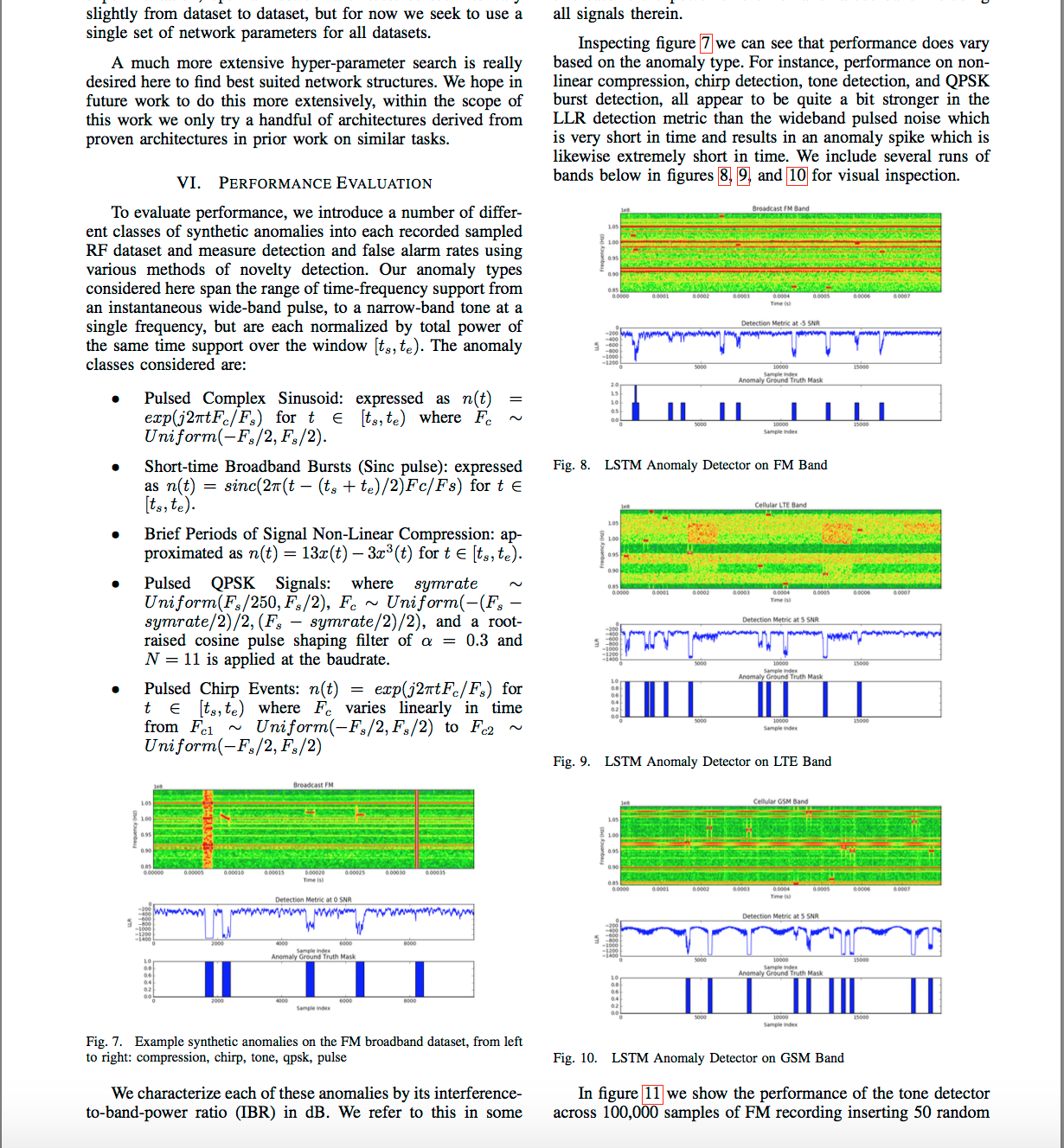
【 事例② 】LSTM モデル を 用いた 異常値検知モデル

LSTM-AD: LSTM-based Anomaly Detection

• Pankaj Malhotra1, Lovekesh Vig, Gautam Shroff, Pundet Agarwal, Long Short Term Memory Networks for Anomaly Detection in Time Series

The rest of the paper is organised as follows: Section 2 describes our ap- proach. In Section 3, we present temporal anomaly detection results on four real-world datasets using our stacked LSTM approach (LSTM-AD) as well as stacked RNN approach using recurrent sigmoid units (RNN-AD). Section 4 offers concluding remarks.

（ モデル模式図。上記の論文 より 転載 ）

（ 結果 ）

• Timothy J. O’Shea, T. Charles Clancy, Robert W. Mcgwire, Recurrent Neural Radio Anomaly Detection

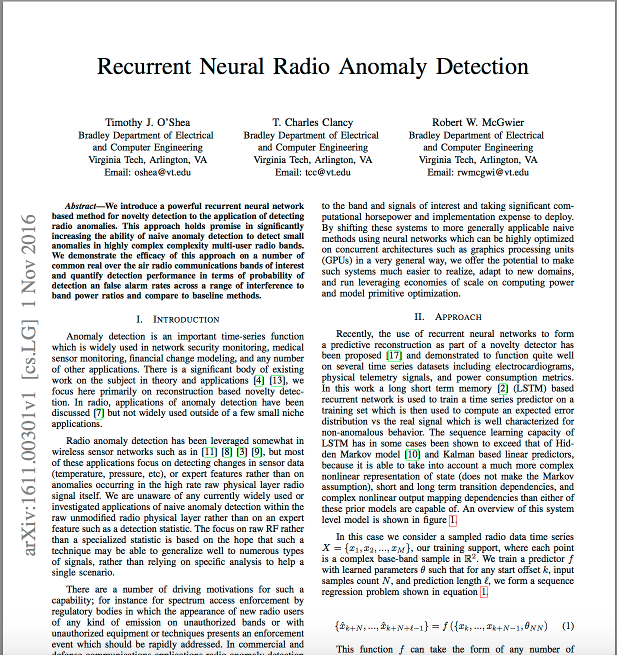
O'Shea氏は、以下の記事で紹介した別の論文でも登場した人と同一人物と思われる。

• HirofumiYashima Qiita記事 「【 国家安全保障 と 深層学習 】変調信号 識別・分類（ELINT, SIGINT, OSINT） に おける 深層学習モデル 活用事例」

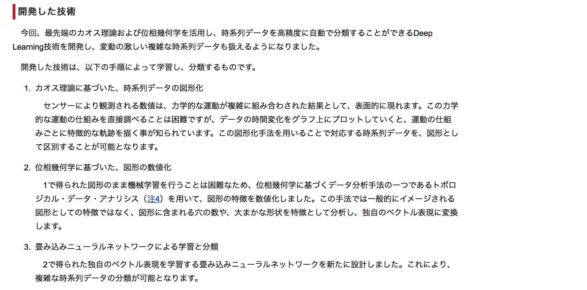
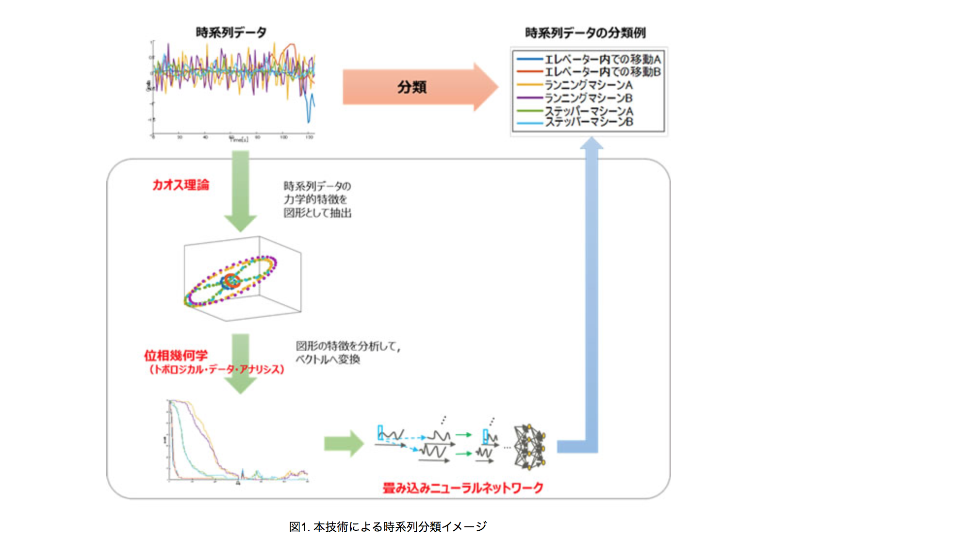
非伝統的アプローチ

時系列データ を plotしたグラフの「形状」がもつ（位相幾何の）特徴情報 を、位相幾何学手法 で 数値ベクトル表現したもの を、CNNの入力層 に 与えて 分類学習する アプローチ

① 時系列データ を グラフ出力
② 位相幾何学 を 用いた手法（TDA） で 数値ベクトル表現化
③ 数値ベクトル を 入力層 に 入れた CNN で 時系列データ を 分類学習

• 株式会社富士通研究所 プレスリリース（2016年2月16日）「時系列データを高精度に分析する新たなDeep Learning技術を開発」

• atmarkIT（2016年02月17日 19時11分 更新）「時系列データの「形状」で分類：トポロジカルデータ分析で時系列データを高精度分析、富士通研究所が開発」, The 30th Annual Conference of the Japanese Society for Artificial Intelligence, 2016

（ その他参考 ）

AutoEncoder, Denoising AutoEncoder について は 以下 が わかりやすい。

• beam2d memo （Dec 23, 2013）「Denoising Autoencoderとその一般化」
• いんふらけいようじょのえにっき （2015/09/16）「chainerでStacked denoting Autoencoder」
• Elix Tech Blog （Jul 17, 2016 ）「Kerasで学ぶAutoencoder」

• まんぼう日記（2015-07-18）「Denoting Autoencoder」の実験をしてみる

• CARL DOERSCH Tutorial on Variational Autoencoders

• nzw「Variational Auto Encoder」

• cympfhさん Qiita記事「Variational Autoencoders (VAEs; 変分オートエンコーダ) (理論)」

• RyotaKatohさん Qiita記事「Variational Autoencoder（VAE）で生成モデル」

• github.com/RyotaKatoh/chainer-Variational-AutoEncoder)

• Use At Your Own Risk (2015/09/01) 「Variational Autoencoderでアルバムジャケットの生成」

• Diederik P. Kingma∗, Danilo J. Rezende†, Shakir Mohamed†, Max Welling, Semi-supervised Learning with Deep Generative Models

• 得居 誠也「論文紹介 Semi-supervised Learning with Deep Generative Models」